6180 CHAPTER 6. THE FREQUENCY-RESPONSE DESIGN METHOD
100101102
10-1
ω (rad/sec)
Bode plot
100101102
10-1
ω (rad/sec)
Bode plot
100101102
-400
0
ω (rad/sec)
100101102
10-1
ω (rad/sec)
Bode plot
100101102
10-1
ω (rad/sec)
Bode plot
100101102
-400
0
ω (rad/sec)
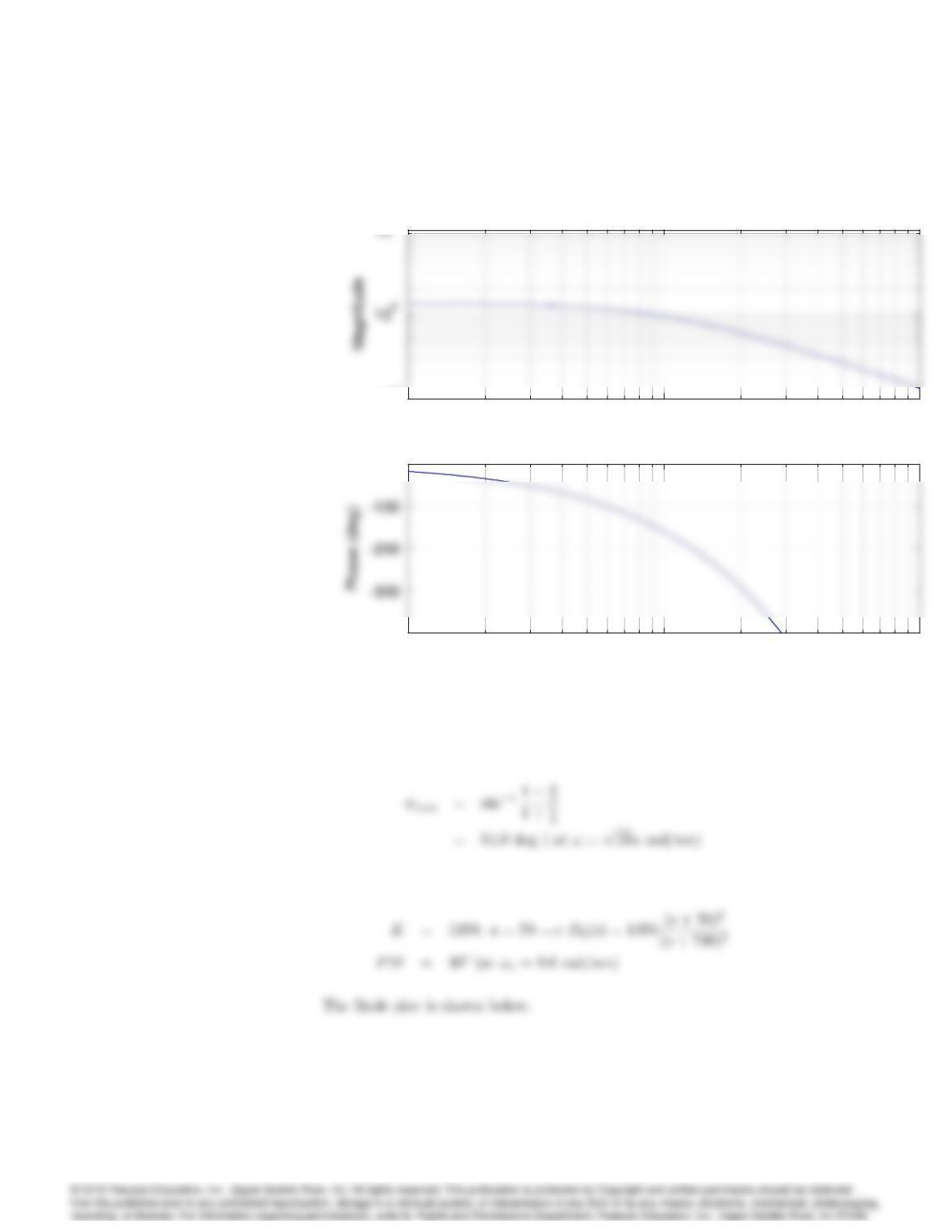
(b) Two lead sections :
With b=a = 10, the lead compensator can add the maximum phase
lead :
By trial and error, one of the possible compensators is :
6181
100101102
10–0.5
100.3
ω (rad/sec)
Bode plot
100101102
10–0.5
100.3
ω (rad/sec)
Bode plot
100101102
-250
0
ω (rad/sec)
100101102
10–0.5
100.3
ω (rad/sec)
Bode plot
100101102
10–0.5
100.3
ω (rad/sec)
Bode plot
100101102
-250
0
ω (rad/sec)
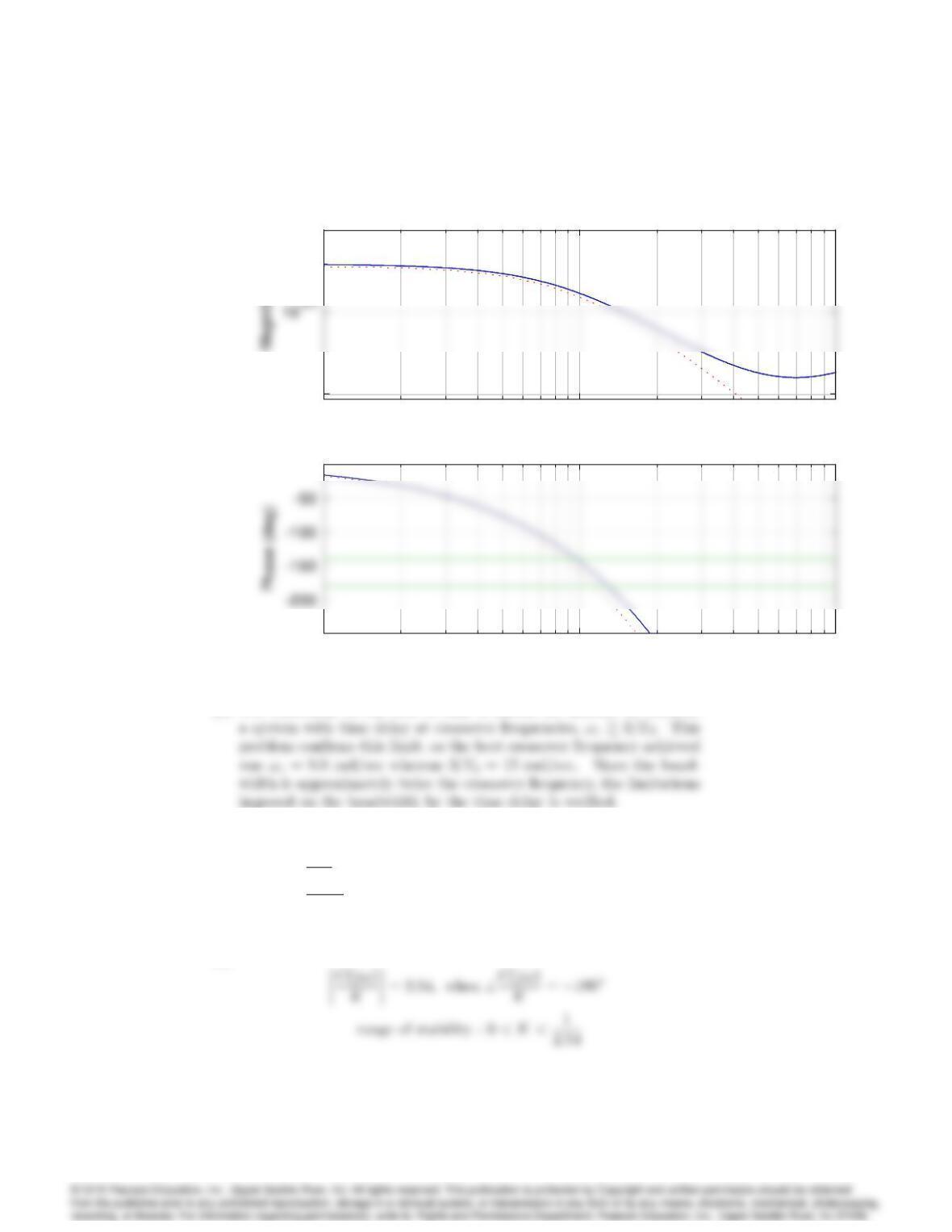
(c) The statement in the text is that it should be difficult to stabilize
65. Determine the range of Kfor which the following systems are stable:
(a) G(s) = Ke4s
s
(b) G(s) = Kes
s(s+2)
Solution :
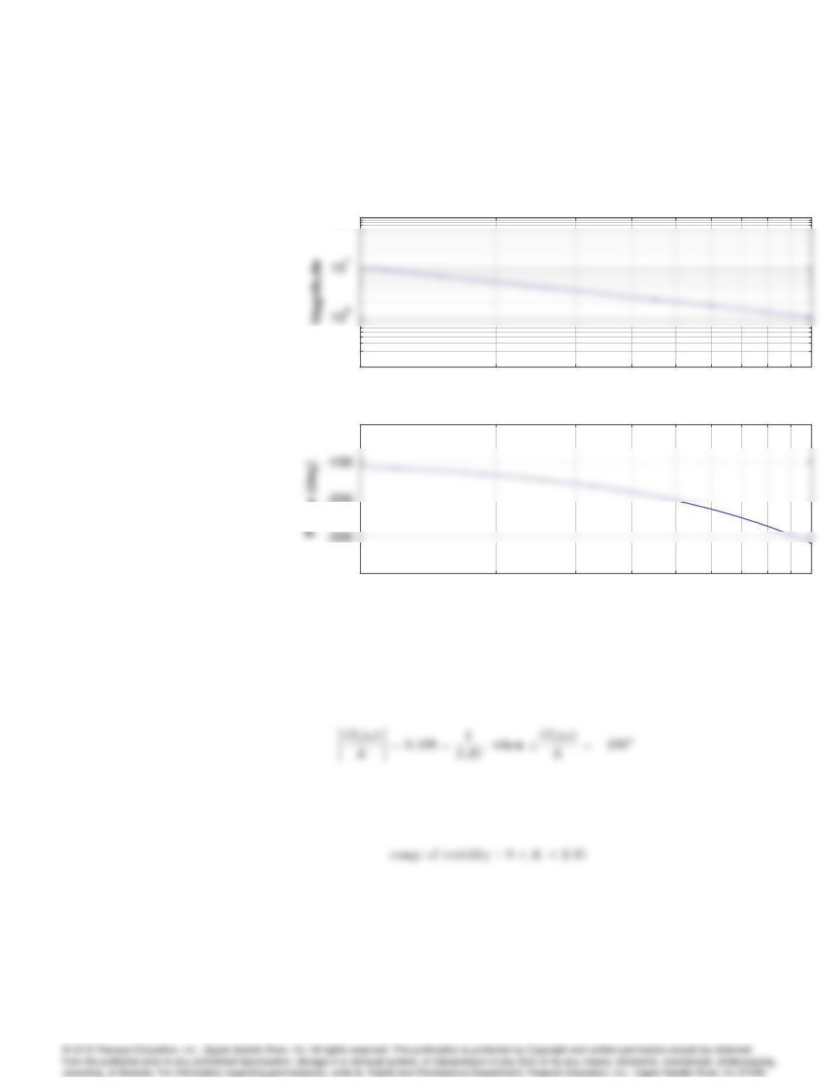
(a)
6182 CHAPTER 6. THE FREQUENCY-RESPONSE DESIGN METHOD
10-1 100
10-1
102
Frequency (rad/sec)
Bode plot
10-1 100
10-1
102
Frequency (rad/sec)
Bode plot
10-1 100
-400
-200
0
ω (rad/sec)
10-1 100
10-1
102
Frequency (rad/sec)
Bode plot
10-1 100
10-1
102
Frequency (rad/sec)
Bode plot
10-1 100
-400
-200
0
ω (rad/sec)
(b)
6183
10-1 100101
101
ω (rad/sec)
Bode plot
10-1 100101
101
ω (rad/sec)
Bode plot
-400
-200
0
10-1 100101
101
ω (rad/sec)
Bode plot
10-1 100101
101
ω (rad/sec)
Bode plot
-400
-200
0
66. Consider the heat exchanger of Example 2.16 with the open-loop transfer
function
G(s) = e5s
(10s+ 1)(60s+ 1):
(a) Design a lead compensator that yields PM 45and the maximum
possible closed-loop bandwidth.
(b) Design a PI compensator that yields PM 45and the maximum
possible closed-loop bandwidth.
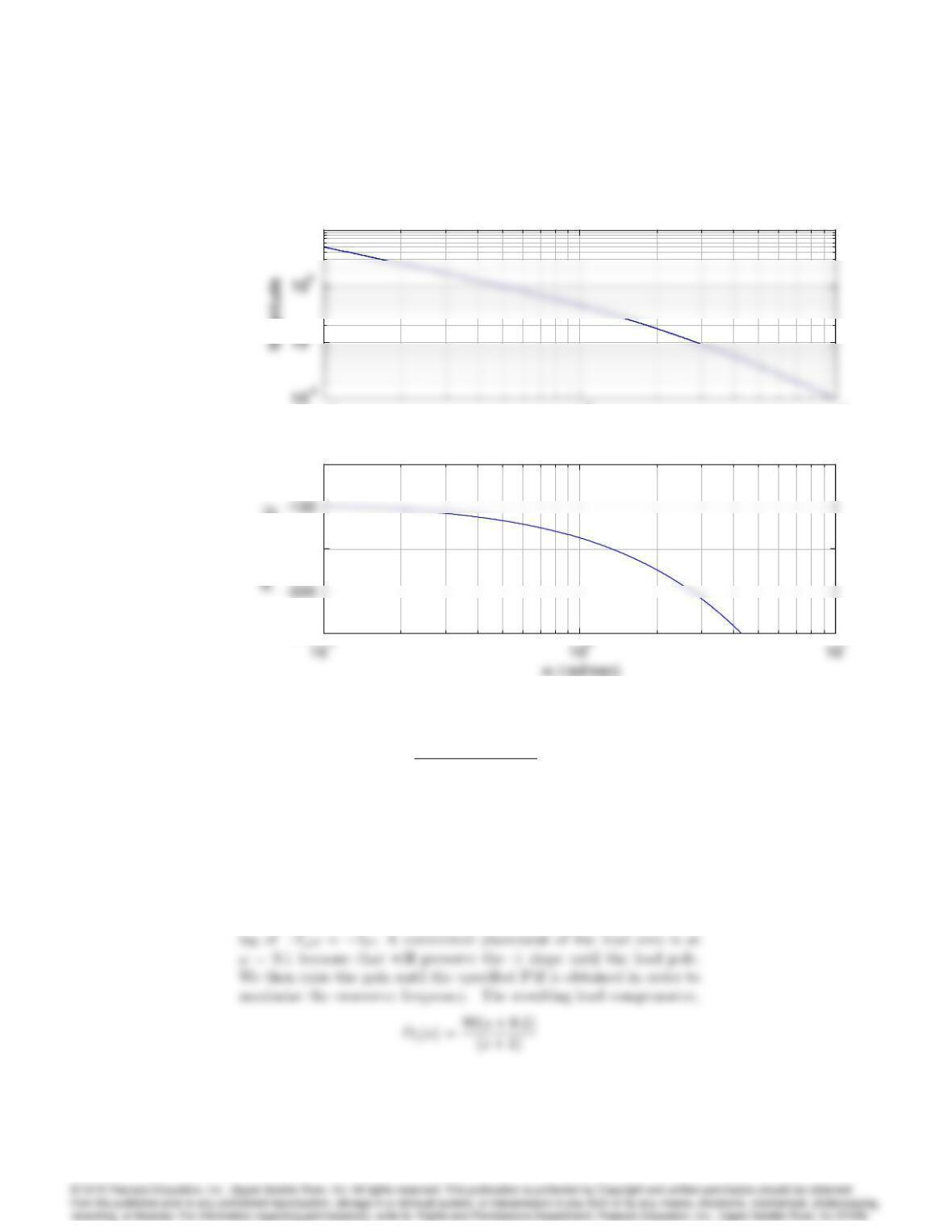
Solution :
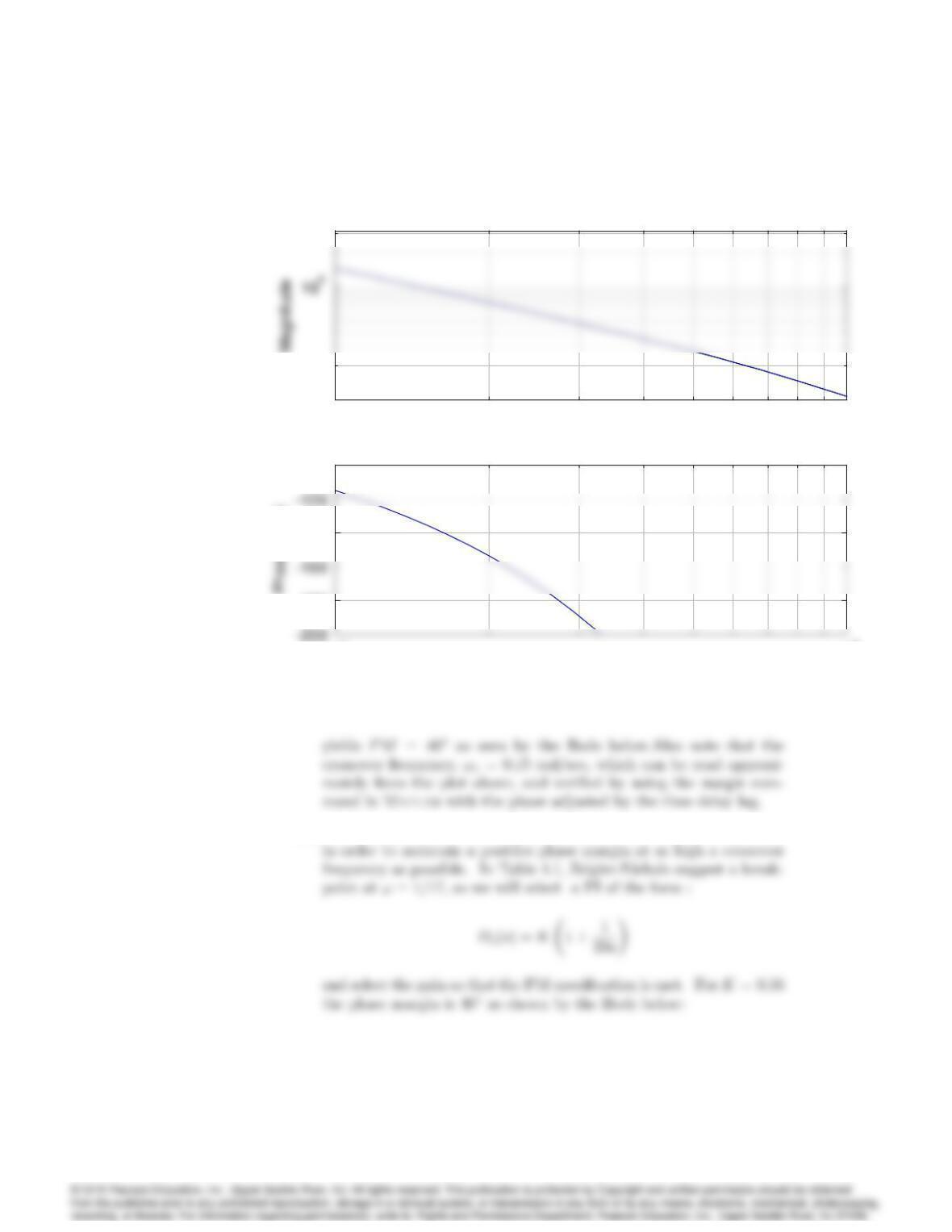
(a) First, make sure that the phase calculation includes the time delay
6184 CHAPTER 6. THE FREQUENCY-RESPONSE DESIGN METHOD
10-1 100
10-1
ω (rad/sec)
Bode plot with Lead Compensation
10-1 100
10-1
ω (rad/sec)
Bode plot with Lead Compensation
10-1 100
-180
-140
-100
ω (rad/sec)
10-1 100
10-1
ω (rad/sec)
Bode plot with Lead Compensation
10-1 100
10-1
ω (rad/sec)
Bode plot with Lead Compensation
10-1 100
-180
-140
-100
ω (rad/sec)
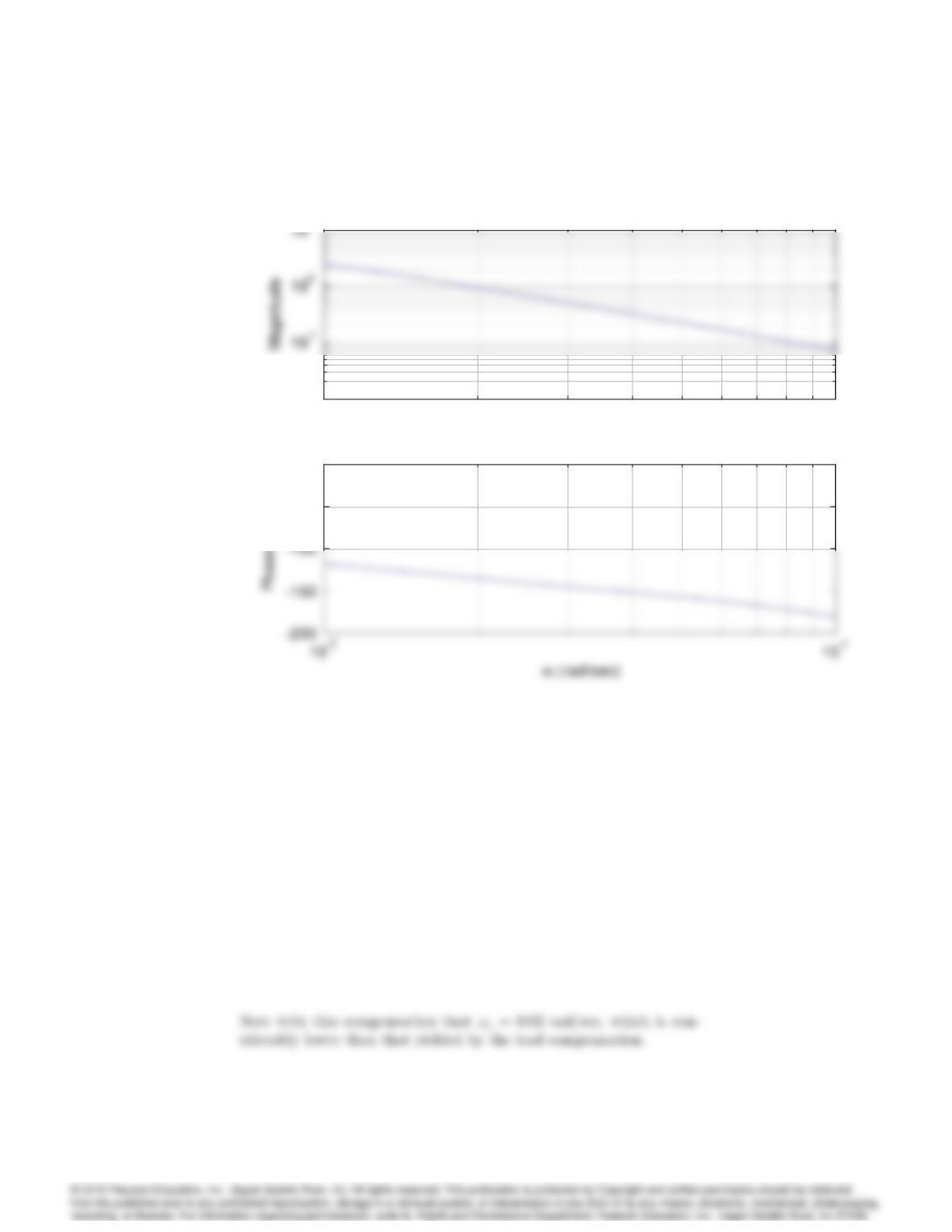
(b) The brealpoint of the PI compensator needs to be kept well below 0.1
6185
10-2 10-1
10-2
ω (rad/sec)
Bode plot with PI compensation
10-2 10-1
10-2
ω (rad/sec)
Bode plot with PI compensation
-50
0
10-2 10-1
10-2
ω (rad/sec)
Bode plot with PI compensation
10-2 10-1
10-2
ω (rad/sec)
Bode plot with PI compensation
-50
0
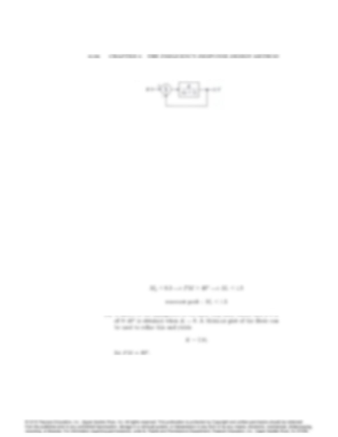
Figure 6.103: Control system for Problem 67
Problems and Solutions for Section 6.9
67. A feedback control system is shown in Fig.6.103. The closed-loop system
is specified to have an overshoot of less than 30% to a step input.
(a) Determine the corresponding PM specification in the frequency do-
main and the corresponding closed-loop resonant peak value Mr. (See
Fig. 6.37)
(b) From Bode plots of the system, determine the maximum value of K
that satisfies the PM specification.
(c) Plot the data from the Bode plots (adjusted by the Kobtained in
part (b)) on a copy of the Nichols chart in Fig. 6.81 and determine the
resonant peak magnitude Mr. Compare that with the approximate
value obtained in part (a).
(d) Use the Nichols chart to determine the resonant peak frequency !r
and the closed-loop bandwidth.
Solution :
(a) From Fig. 6.37 :
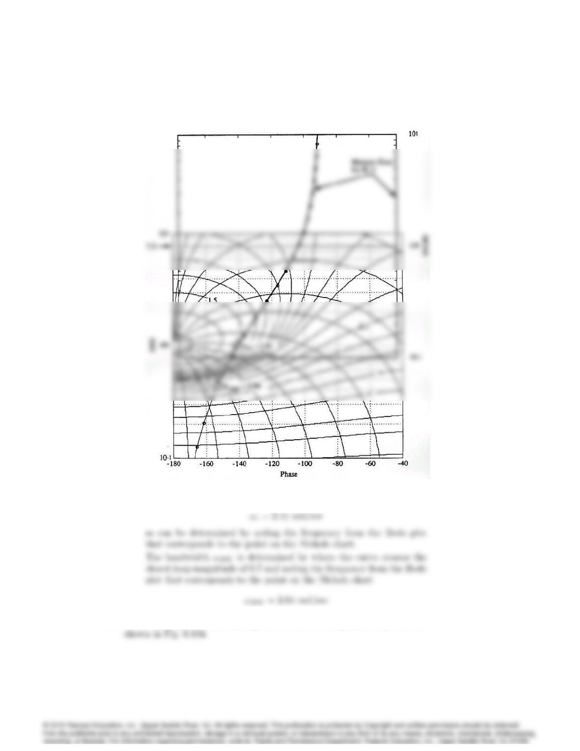
(c) The Nichols chart below shows that Mr= 1:5which agrees exactly
with the prediction from Fig. 6.37:
6187
(d) The corresponding frequency where the curve is tangent to Mr= 1:5
is:
68. The Nichols plot of an uncompensated and a compensated system are
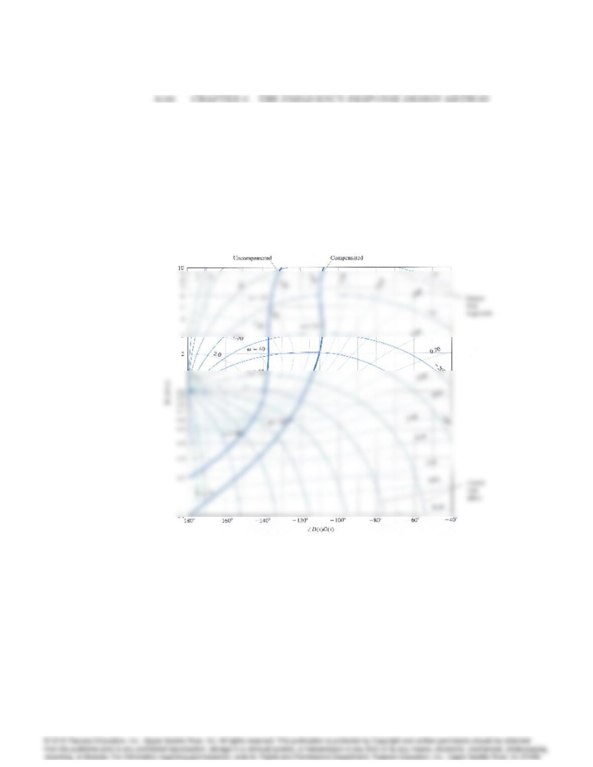
Figure 6.104: Nichols plot for Problem 68
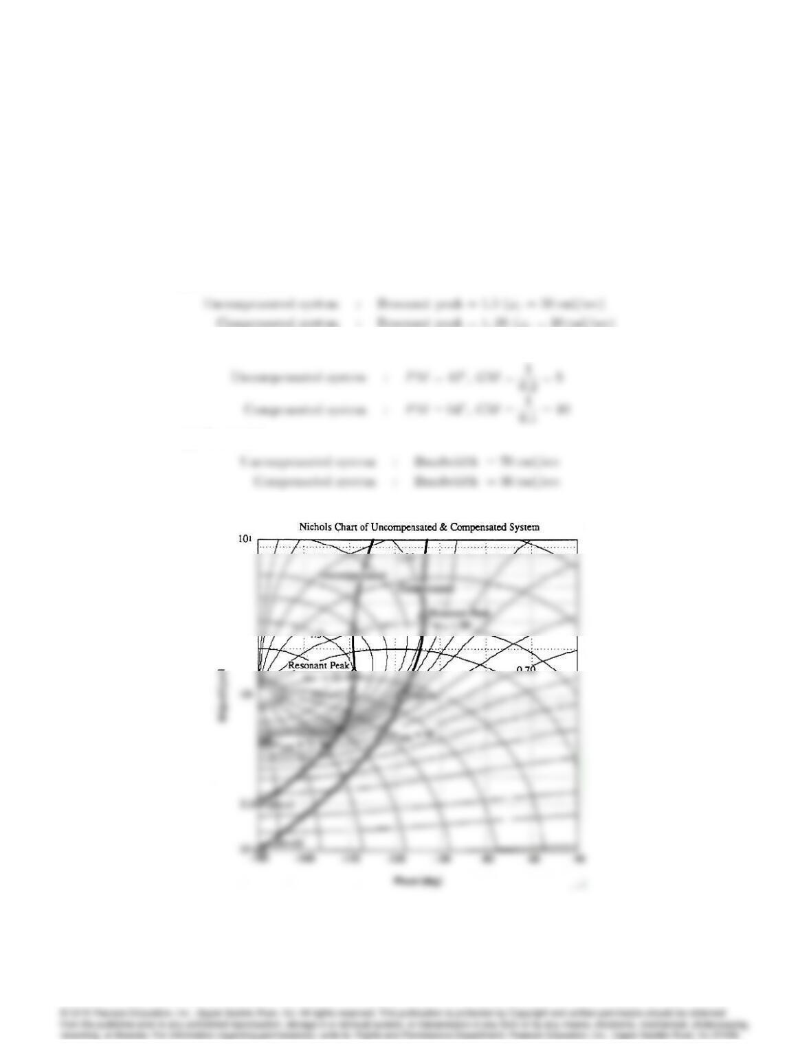
6189
(a) What are the resonance peaks of each system?
(b) What are the PM and GM of each system?
(c) What are the bandwidths of each system?
(d) What type of compensation is used?
Solution :
(a) Resonant peak :
Compensated system :Resonant peak = 1::05 (!r= 20 rad/sec)
(b) PM, GM :
(c) Bandwidth :
(d) Lag compensation is used, since the bandwidth is reduced.
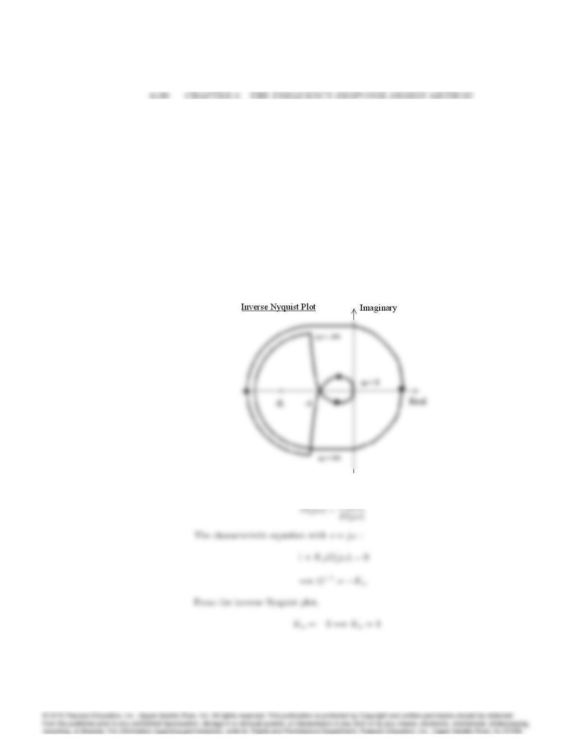
69. Consider the system shown in Fig. 6.95.
(a) Construct an inverse Nyquist plot of [Y(j!)=E(j!)]1. (See Ap-
pendix W6.9.2)
(b) Show how the value of Kfor neutral stability can be read directly
from the inverse Nyquist plot.
(c) For K= 4, 2, and 1, determine the gain and phase margins.
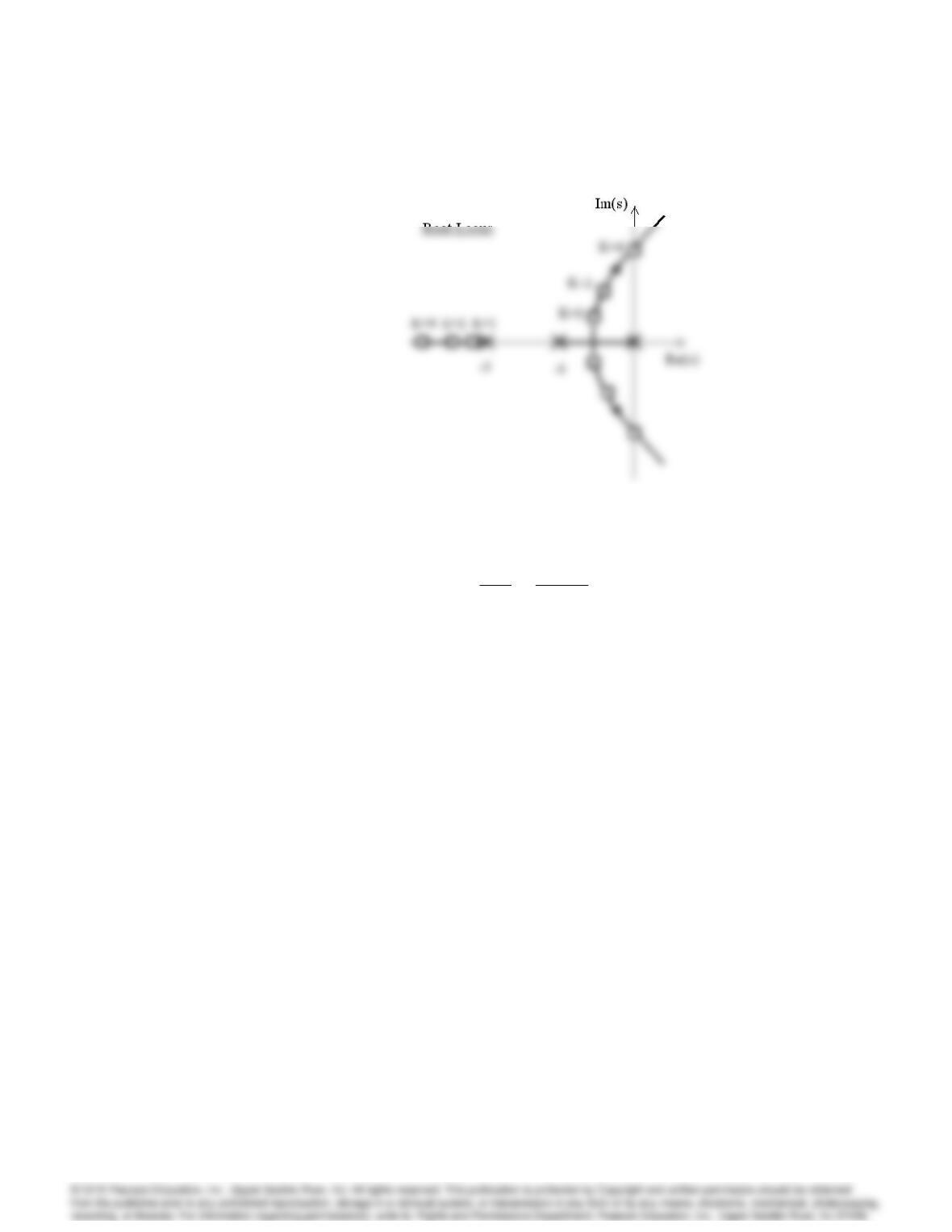
(d) Construct a root-locus plot for the system, and identify corresponding
points in the two plots. To what damping ratios do the GM and
PM of part (c) correspond?
Solution :
(a) See the inverse Nyquist plot.
(b) Let
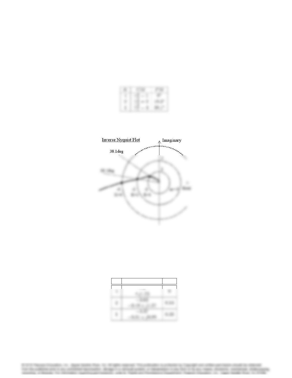
6191
(c)
(d)
Kclosed-loop poles
6192 CHAPTER 6. THE FREQUENCY-RESPONSE DESIGN METHOD
70. An unstable plant has the transfer function
Y(s)
F(s)=s+ 1
(s1)2:
A simple control loop is to be closed around it, in the same manner as the
block diagram in Fig. 6.95.
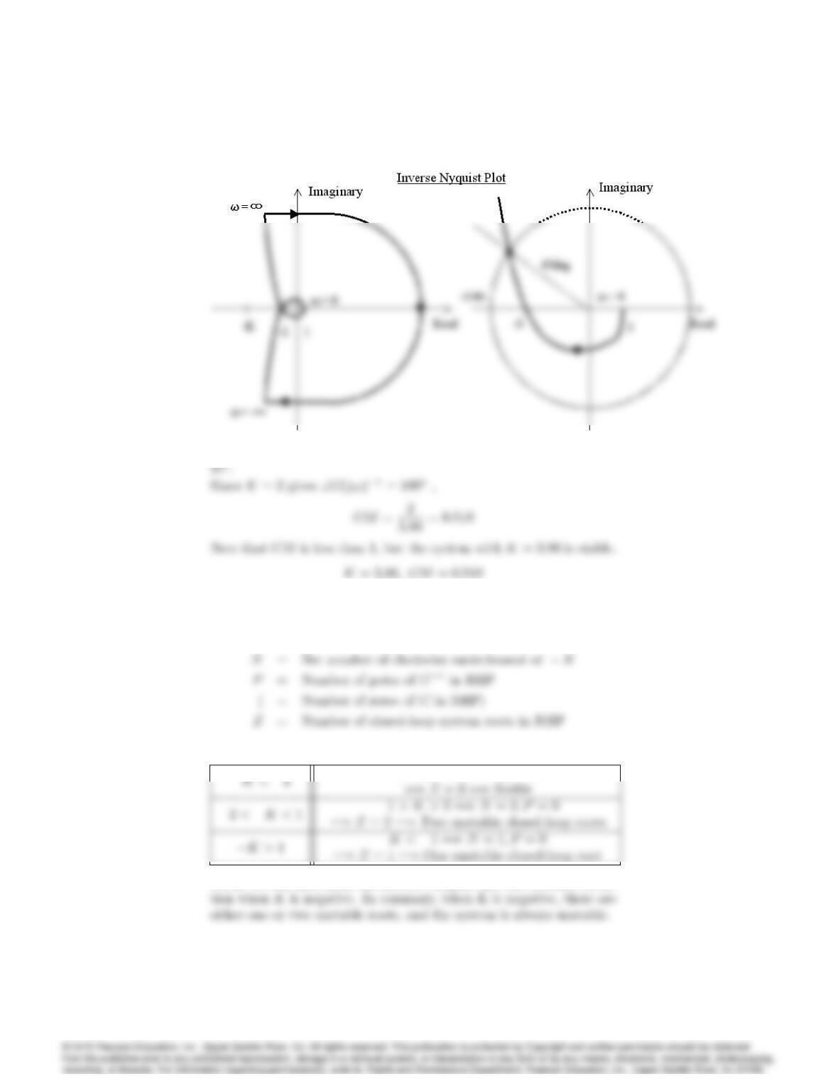
(a) Construct an inverse Nyquist plot of Y=F . (See Appendix W6.9.2)
(b) Choose a value of Kto provide a PM of 45. What is the corre-
sponding GM?
(c) What can you infer from your plot about the stability of the system
when K < 0?
(d) Construct a root-locus plot for the system, and identity correspond-
ing points in the two plots. In this case, to what value of does
PM = 45correspond?
Solution :
(a) The plots are :
6193
(b) From the inverse Nyquist plot, K= 3:86 provides a phase margin of
(c) We can apply stability criteria to the inverse Nyquist plot as follows
:
Let
Then,
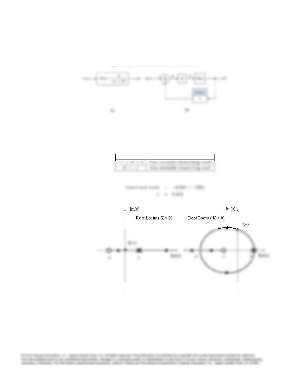
Then, we can infer from the inverse Nyquist plot the stability situa-
6194 CHAPTER 6. THE FREQUENCY-RESPONSE DESIGN METHOD
Figure 6.105: Control system for Problem 71
(d) The stability situation seen in the root locus plot agrees with that
obtained from the inverse Nyquist plot.
They show :
K > 2Stable
For the phase margin 45,
71. Consider the system shown in Fig. 6.105(a).
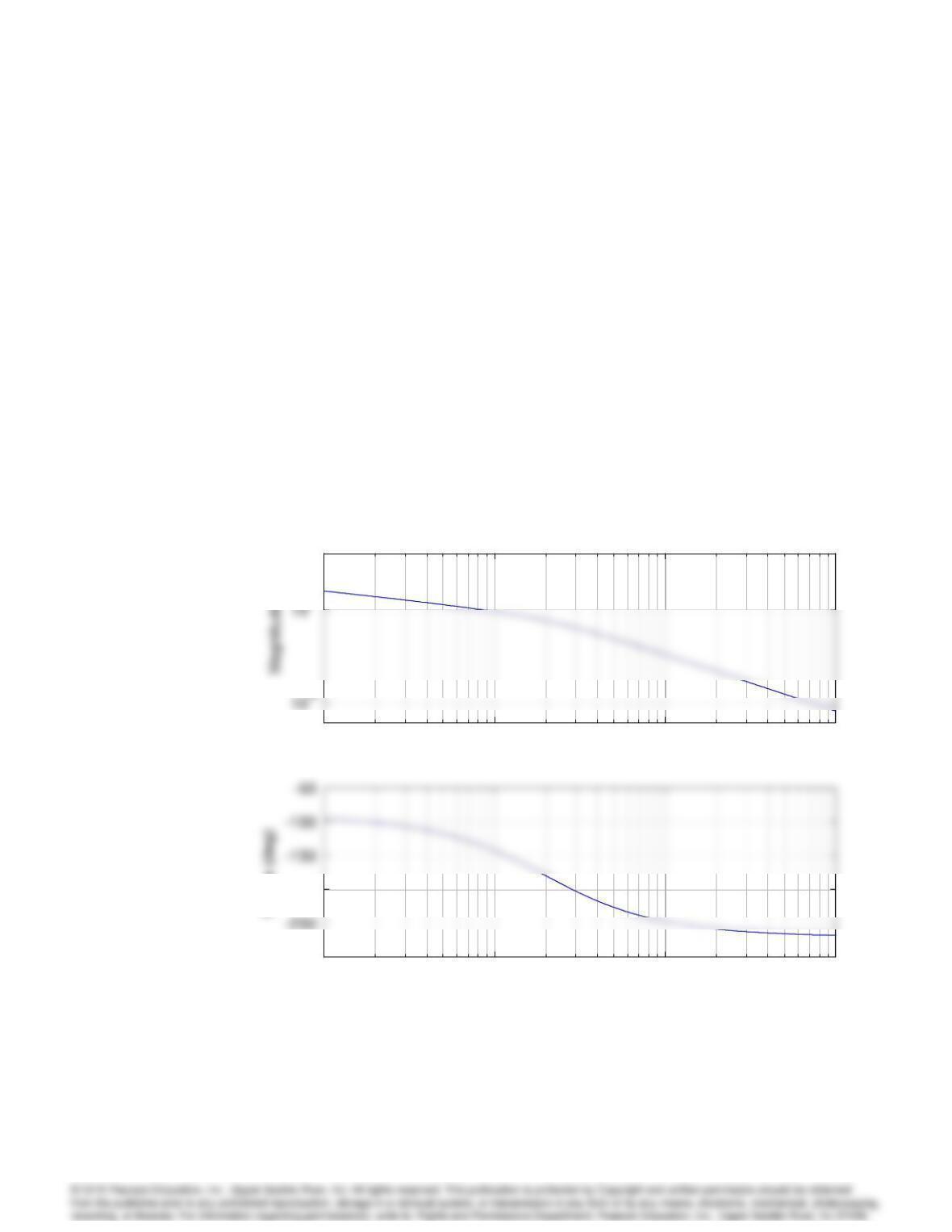
(a) Construct a Bode plot for the system.
6195
(b) Use your Bode plot to sketch an inverse Nyquist plot. (See Appendix
W6.9.2)
(c) Consider closing a control loop around G(s), as shown in Fig. 6.105(b).
Using the inverse Nyquist plot as a guide, read from your Bode plot
the values of GM and PM when K= 0:7, 1.0, 1.4, and 2. What value
of Kyields PM = 30?
(d) Construct a root-locus plot, and label the same values of Kon the
locus. To what value of does each pair of PM/GM values corre-
spond? Compare the vs PM with the rough approximation in Fig.
6.36
Solution :
(a) The figure follows, with K = 1. :
10-1 100101102
ω (rad/sec)
Bode Diagrams
10-1 100101102
-300
-200
ω (rad/sec)
Phase (deg)
10-1 100101102
ω (rad/sec)
Bode Diagrams
10-1 100101102
-300
-200
ω (rad/sec)
Phase (deg)
(b) The Inverse Nyquist is:
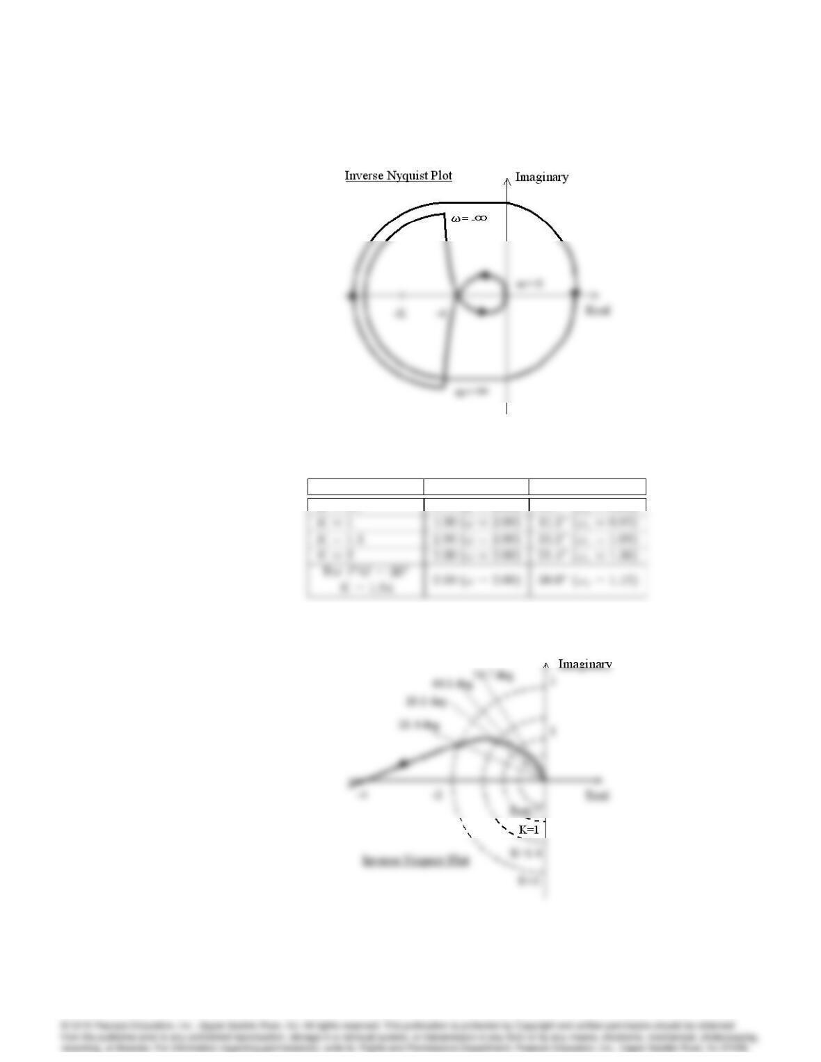
6196 CHAPTER 6. THE FREQUENCY-RESPONSE DESIGN METHOD
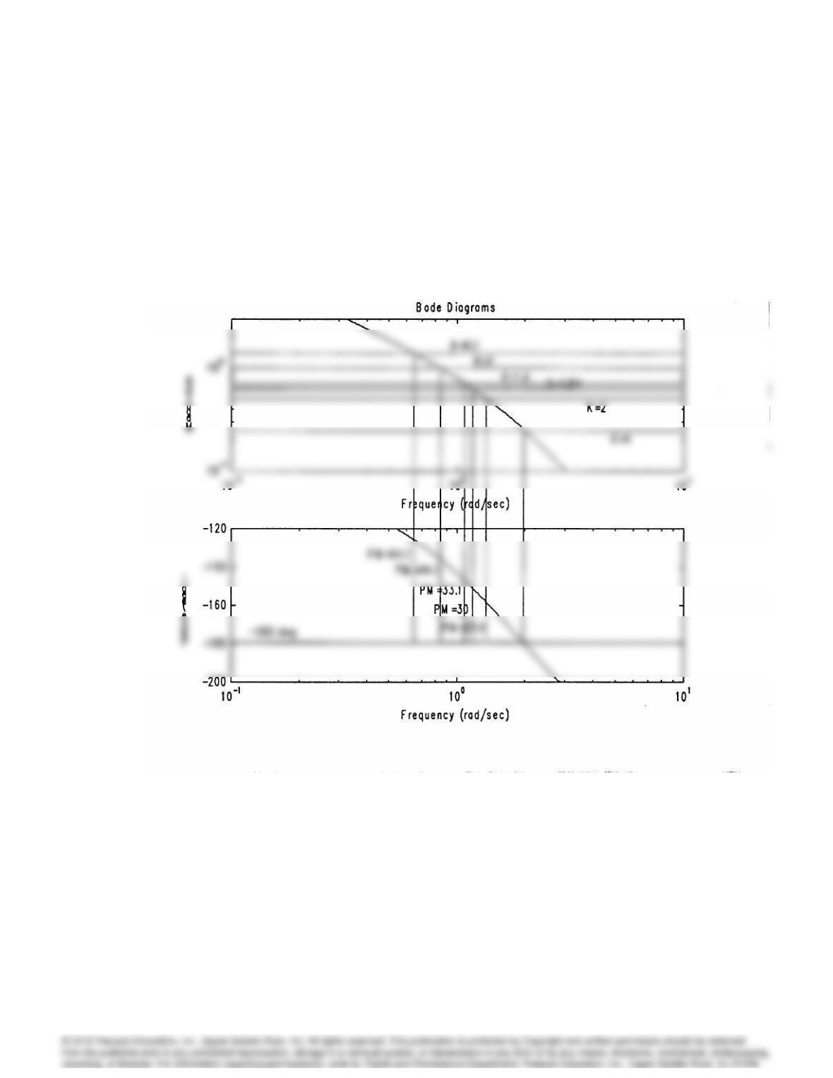
(c) With guidance from the Inverse Nyquist, we can use Matlab’s margin
command to find:ng
K GM P M
K= 0:7 5:71 (!= 2:00) 54:7(!c= 0:64)
and then looking at the Bode, we can interpolate to fgure out what
K would yield the desired 30 Deg PM, as seen below:
6197
6198 CHAPTER 6. THE FREQUENCY-RESPONSE DESIGN METHOD
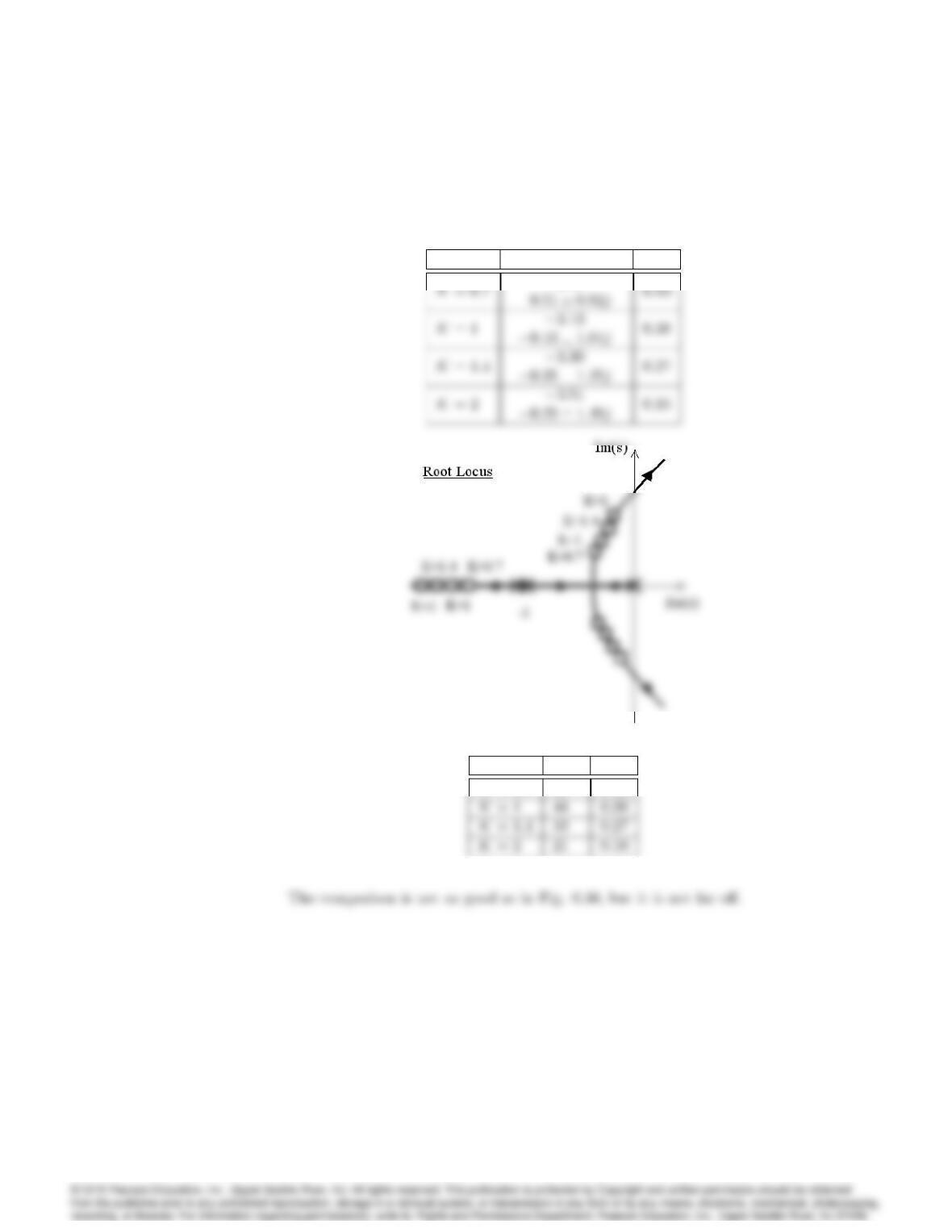
(d) Now we take a look at the RL, but expediting the detailed value of
by using Matlab’s damp with the various values of K in the feeedback
loop.
Kclosed-loop roots
K P M
K= 0:7 55 0:53