6160 CHAPTER 6. THE FREQUENCY-RESPONSE DESIGN METHOD
–100
–60
–20
Magnitude (dB)
10
-4
10
-3
10
-2
10
-1
10
0
10
1
10
2
–270
–90
Bode Diagram
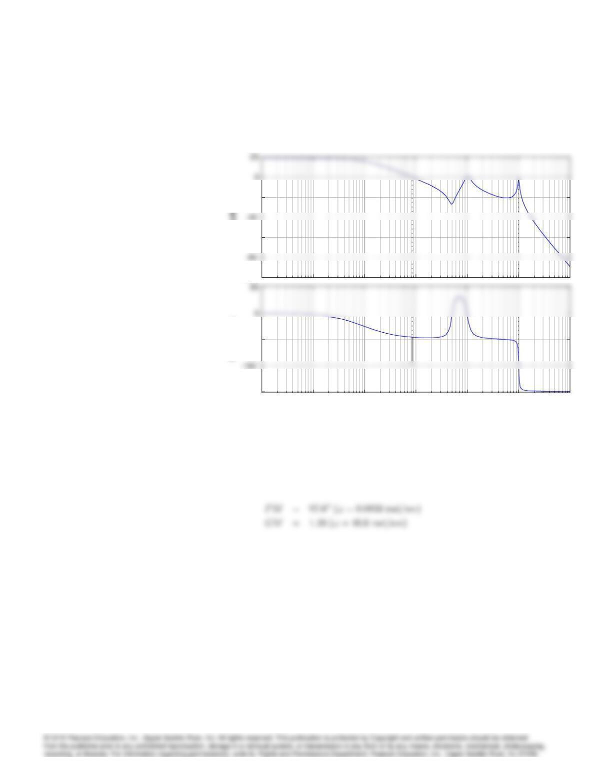
Gm = 1.28 dB (at 10 rad/sec) , Pm = 97.6 deg (at 0.0833 rad/sec)
Frequency (rad/sec)
–100
–60
–20
Magnitude (dB)
10
-4
10
-3
10
-2
10
-1
10
0
10
1
10
2
–270
–90
The low GM is caused by the resonance being close to instability.
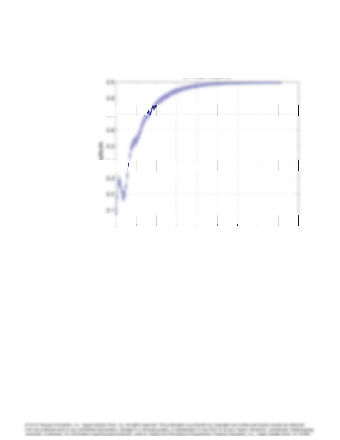
The closed-loop system unit step response is :
6161
010 20 30 40 50 60 70 80 90
0
0.4
Time (sec)
Amplitude
010 20 30 40 50 60 70 80 90
0
0.4
Time (sec)
Amplitude
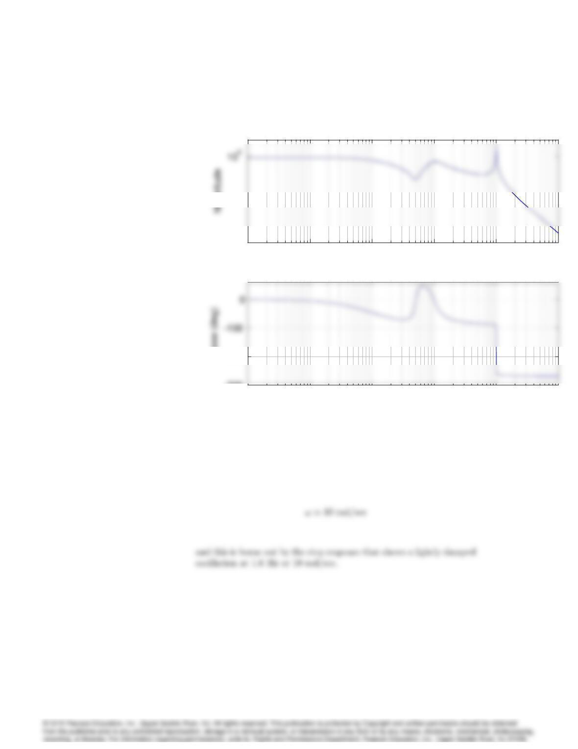
The Bode plot of the closed-loop system is :
6162 CHAPTER 6. THE FREQUENCY-RESPONSE DESIGN METHOD
10-3 10-2 10-1 100101102
10-5
ω (rad/sec)
Bode plot
10-3 10-2 10-1 100101102
10-5
ω (rad/sec)
Bode plot
10-3 10-2 10-1 100101102
-300
-200
ω (rad/sec)
Phase (deg)
10-3 10-2 10-1 100101102
10-5
ω (rad/sec)
Bode plot
10-3 10-2 10-1 100101102
10-5
ω (rad/sec)
Bode plot
10-3 10-2 10-1 100101102
-300
-200
ω (rad/sec)
Phase (deg)
From the Bode plot of the closed -loop system, the frequency of the
lightly damped mode is :
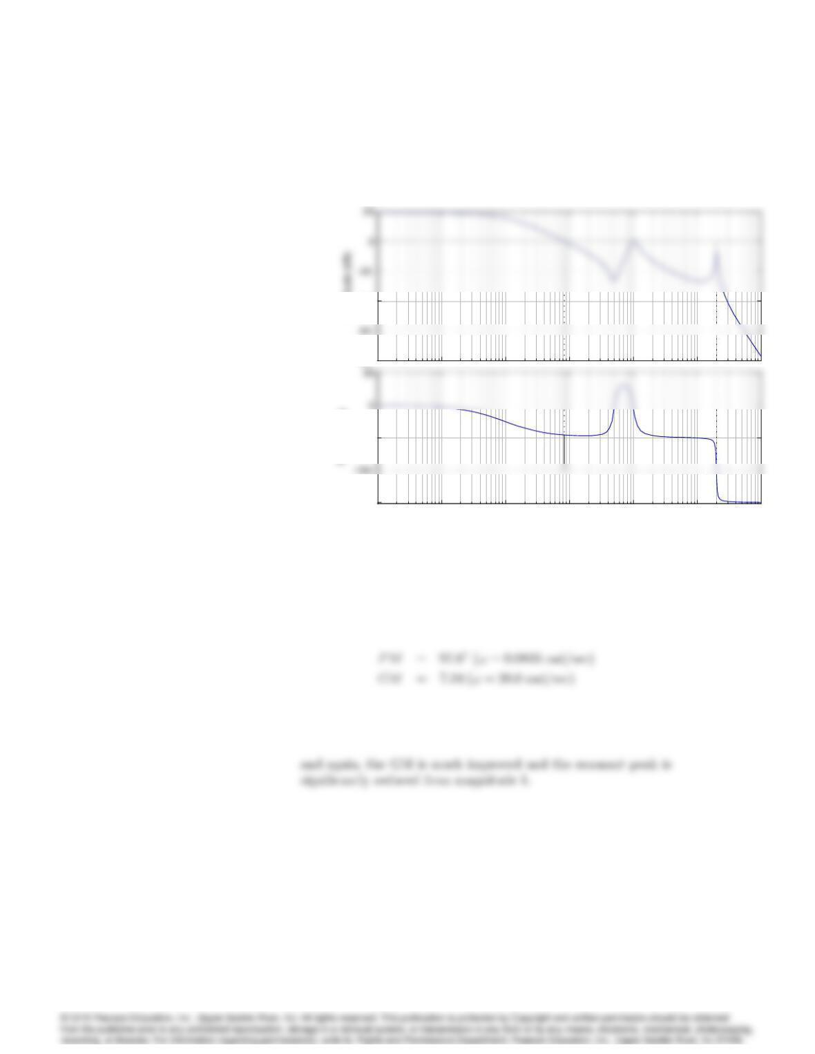
i. The Bode plot of the system with the bending mode damping
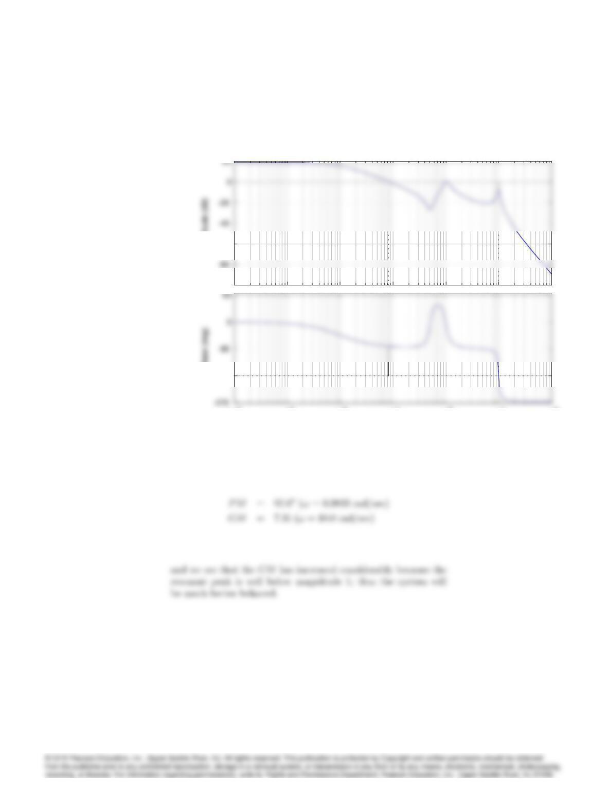
increased from = 0:02 to = 0:04 is :
6163
–100
–60
Magnitude (dB)
10
-4
10
-3
10
-2
10
-1
10
0
10
1
10
2
–180
Phase (deg)
Bode Diagram
Gm = 7.31 dB (at 10 rad/sec) , Pm = 97.6 deg (at 0.0833 rad/sec)
Frequency (rad/sec)
–100
–60
Magnitude (dB)
10
-4
10
-3
10
-2
10
-1
10
0
10
1
10
2
–180
Phase (deg)
ii. The Bode plot of this system (!b= 10 rad/sec =)!b= 20
rad/sec) is :
6164 CHAPTER 6. THE FREQUENCY-RESPONSE DESIGN METHOD
–80
–40
Magnitude (dB)
10-4 10-3 10-2 10-1 100101102
–270
–90
Bode Diagram
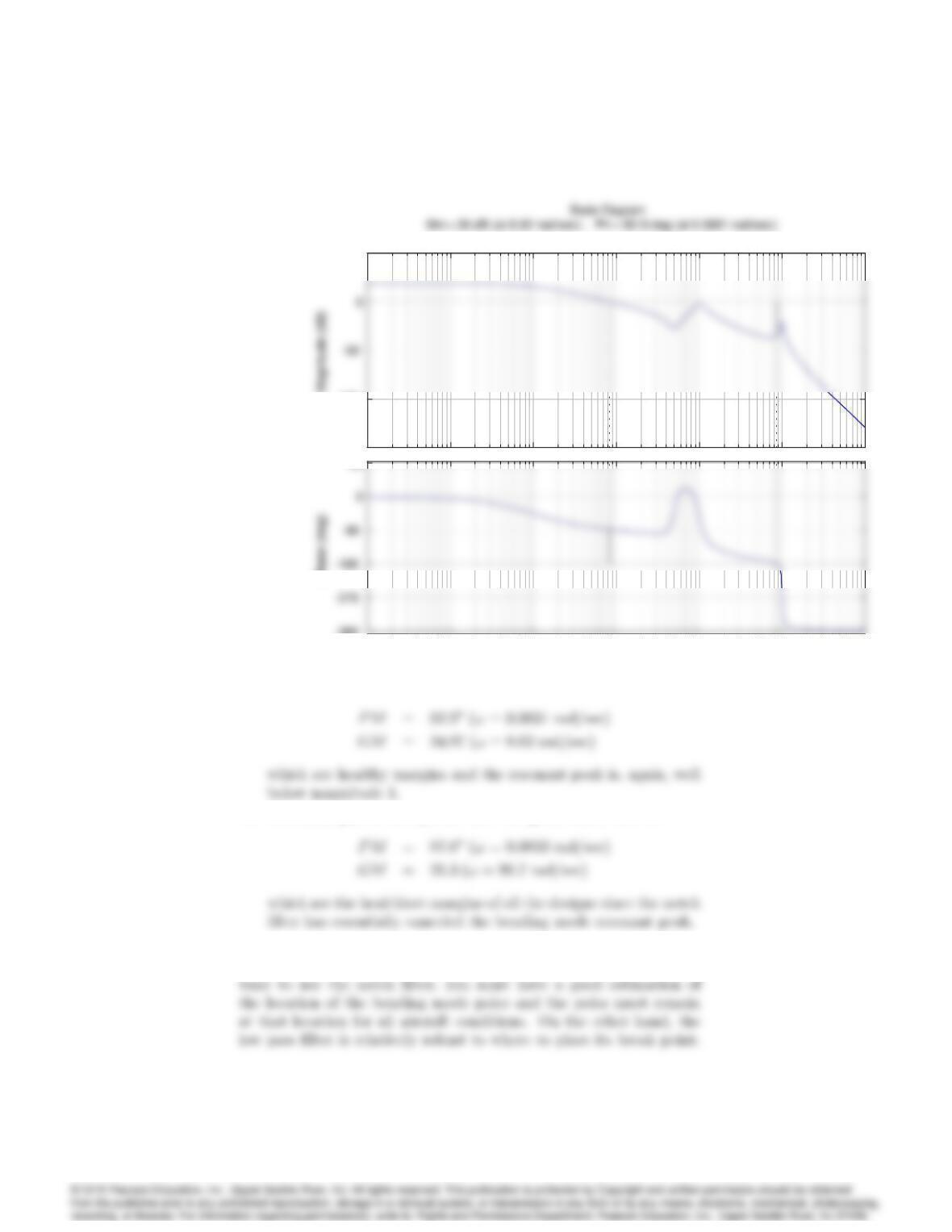
Gm = 7.35 dB (at 20 rad/sec) , Pm = 97.6 deg (at 0.0833 rad/sec)
Frequency (rad/sec)
–80
–40
Magnitude (dB)
10-4 10-3 10-2 10-1 100101102
–270
–90
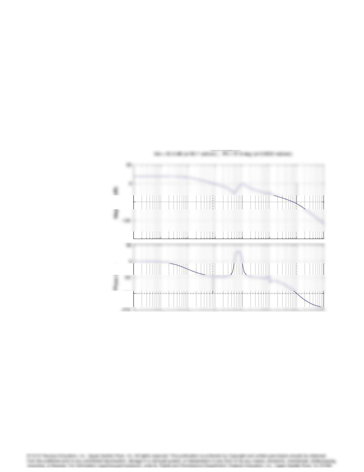
iii. By picking up p= 1;the Bode plot of the system with the low
pass filter is :
6165
–150
–100
50
Magnitude (dB)
10
-4
10
-3
10
-2
10
-1
10
0
10
1
10
2
–360
90
Phase (deg)
Frequency (rad/sec)
–150
–100
50
Magnitude (dB)
10
-4
10
-3
10
-2
10
-1
10
0
10
1
10
2
–360
90
Phase (deg)
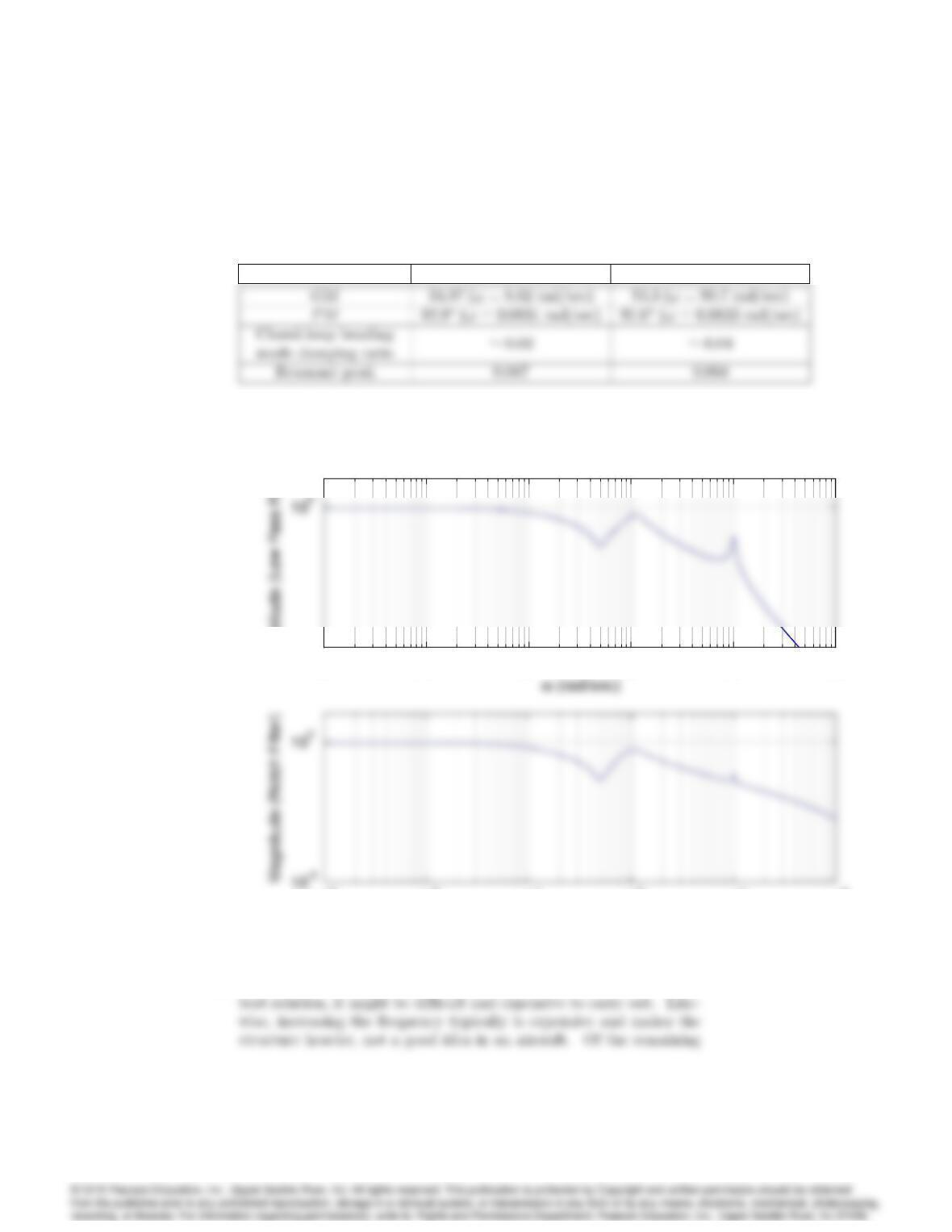
iv. The Bode plot of the system with the given notch filter is :
(b) Generally, the notch filter is very sensitive to where to place the notch
zeros in order to reduce the lightly damped resonant peak. So if you
6166 CHAPTER 6. THE FREQUENCY-RESPONSE DESIGN METHOD
–150
–50
10
-4
10
-3
10
-2
10
-1
10
0
10
1
10
2
10
3
–180
Frequency (rad/sec)
–150
–50
10
-4
10
-3
10
-2
10
-1
10
0
10
1
10
2
10
3
–180
6167
Evaluation of the margins with the bending mode frequency lowered
by 10% will show a drastic reduction in the margins for the notch
filter and very little reduction for the low pass filter.
Low Pass Filter Notch Filter
The magnitude plots of the closed-loop systems are :
10-3 10-2 10-1 100101102
10-5
Magnitude (Low Pass Filter)
Bode plot
10-3 10-2 10-1 100101102
10-5
Magnitude (Low Pass Filter)
Bode plot
10-3 10-2 10-1 100101102
ω (rad/sec)
10-3 10-2 10-1 100101102
10-5
Magnitude (Low Pass Filter)
Bode plot
10-3 10-2 10-1 100101102
10-5
Magnitude (Low Pass Filter)
Bode plot
10-3 10-2 10-1 100101102
ω (rad/sec)
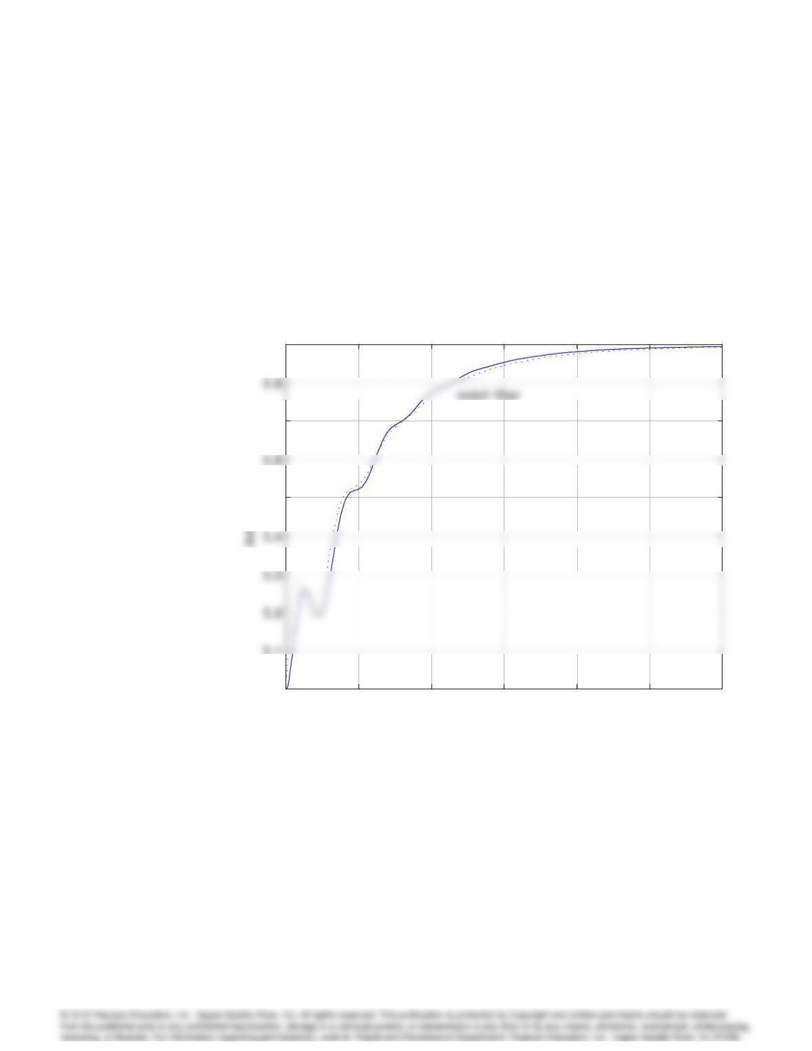
The closed-loop step responses are :
(c) While increasing the natural damping of the system would be the
6168 CHAPTER 6. THE FREQUENCY-RESPONSE DESIGN METHOD
010 20 30 40 50 60
0
0.1
0.5
0.7
0.9
Time (sec)
Unit Step Response
010 20 30 40 50 60
0
0.1
0.5
0.7
0.9
Time (sec)
Unit Step Response
low pass filter
60. Consider a system with the open-loop transfer function (loop gain)
G(s) = 1
s(s+ 1)(s=10 + 1):
(a) Create the Bode plot for the system, and find GM and PM.
(b) Compute the sensitivity function and plot its magnitude frequency
response.
(c) Compute the Vector Margin (VM).
Solution :
(a) The Bode plot is :
10-2 10-1 100101102
10-5
Frequency (rad/sec)
Bode plot
10-2 10-1 100101102
10-5
Frequency (rad/sec)
Bode plot
10-2 10-1 100101102
-250
-50
Frequency (rad/sec)
10-2 10-1 100101102
10-5
Frequency (rad/sec)
Bode plot
10-2 10-1 100101102
10-5
Frequency (rad/sec)
Bode plot
10-2 10-1 100101102
-250
-50
Frequency (rad/sec)
6170 CHAPTER 6. THE FREQUENCY-RESPONSE DESIGN METHOD
(b) Sensitivity function is :
10 + 1)
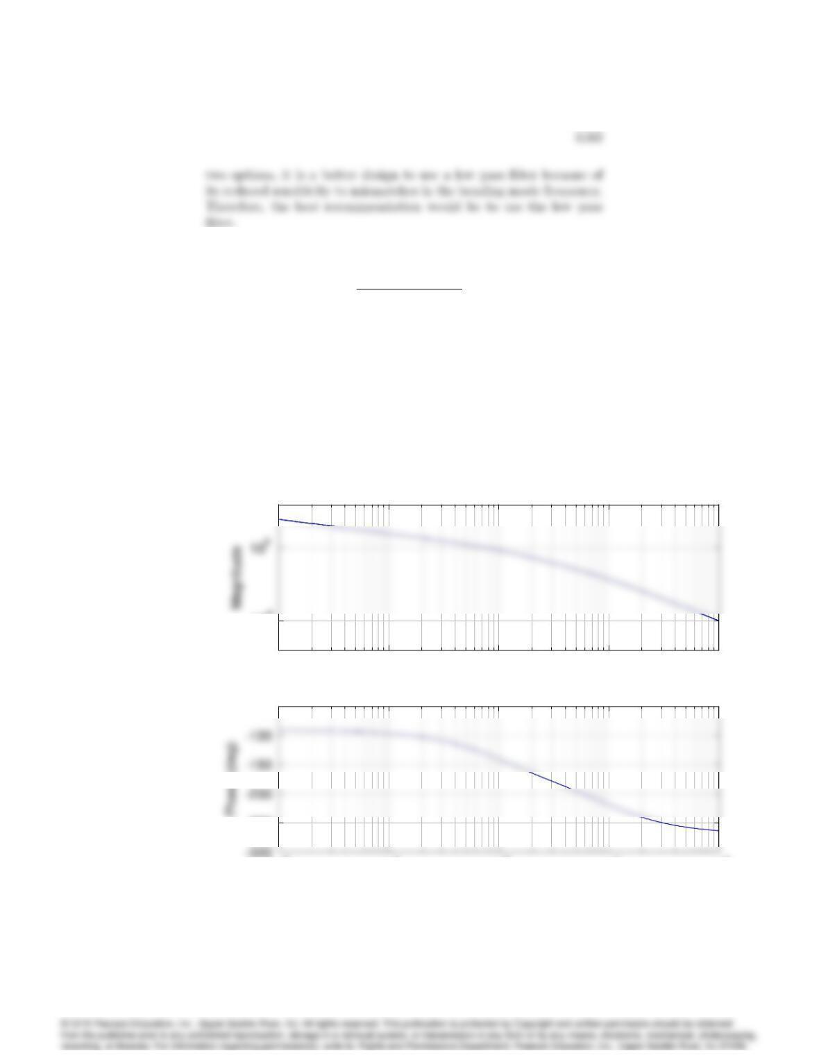
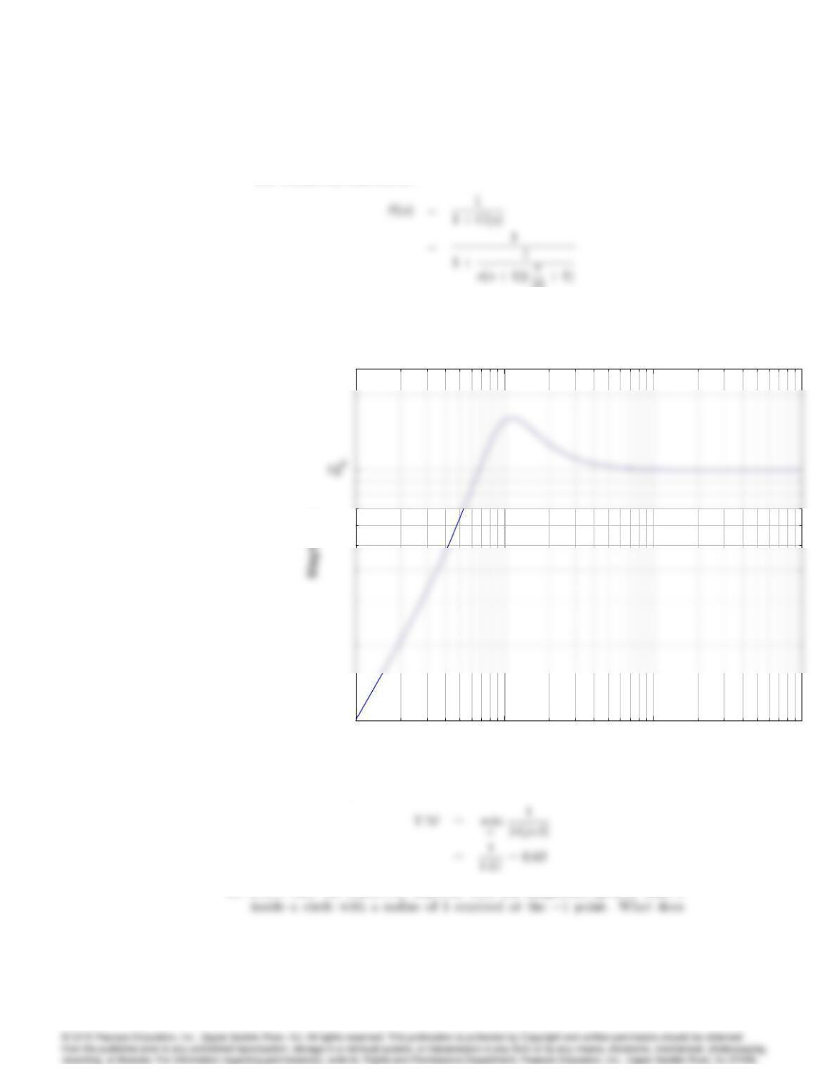
The magnitude frequency response of this sensitivity function is :
10-1 100101102
10-1
ω (rad/sec)
Frequency Response of the Sensitivity Function
10-1 100101102
10-1
ω (rad/sec)
Frequency Response of the Sensitivity Function
(c) Vector Margin is defined as :
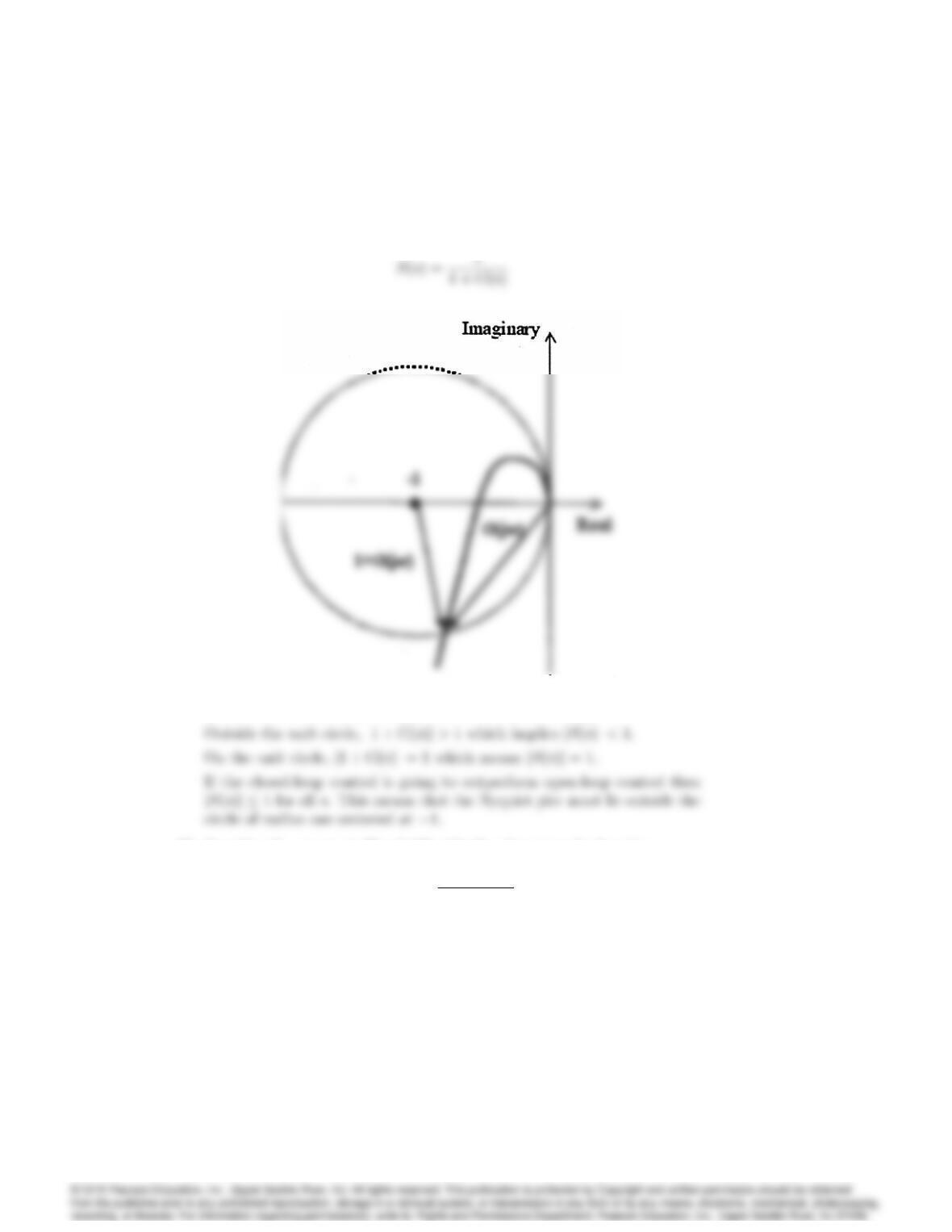
61. Prove that the sensitivity function S(s)has magnitude greater than 1
6171
this imply about the shape of the Nyquist plot if closed-loop control is to
outperform open-loop control at all frequencies?
Solution :
Inside the unit circle, j1 + G(s)j<1which implies jS(s)j>1.
62. Consider the system in Fig. 6.100 with the plant transfer function
G(s) = 10
s(s=10 + 1):
We wish to design a compensator D(s)that satisfies the following design
specifications:
(a) i. Kv= 100,
ii. PM 45,
iii. sinusoidal inputs of up to 1 rad/sec to be reproduced with 2%
error,
6172 CHAPTER 6. THE FREQUENCY-RESPONSE DESIGN METHOD
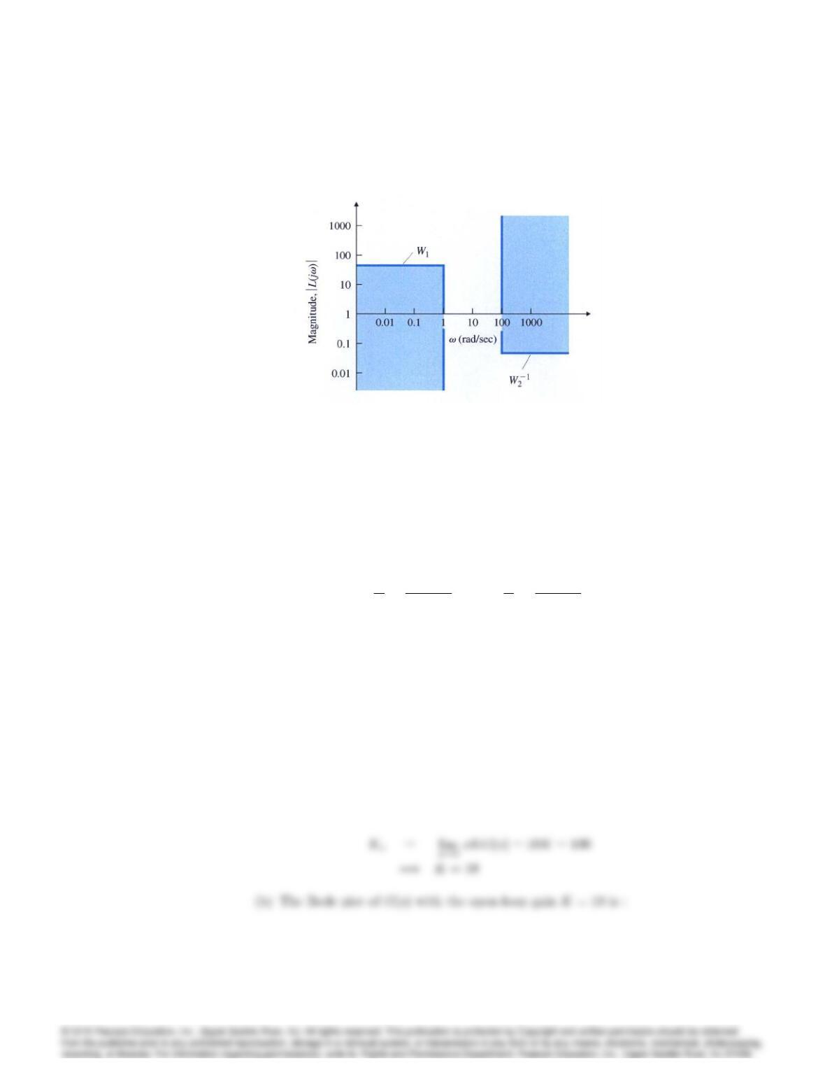
Figure 6.102: Control system constraints for Problem 62
iv. sinusoidal inputs with a frequency of greater than 100 rad/sec to
be attenuated at the output to 5% of their input value.
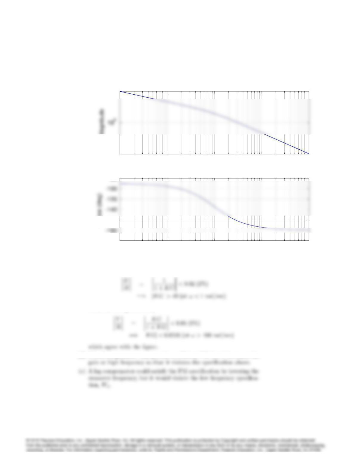
(b) Create the Bode plot of G(s), choosing the open-loop gain so that
Kv= 100.
(c) Show that a sufficient condition for meeting the specification on si-
nusoidal inputs is that the magnitude plot lies outside the shaded
regions in Fig. 6.102. Recall that
Y
R=KG
1 + KG and E
R=1
1 + KG :
(d) Explain why introducing a lead network alone cannot meet the design
specifications.
(e) Explain why a lag network alone cannot meet the design specifica-
tions.
(f) Develop a full design using a lead-lag compensator that meets all
the design specifications, without altering the previously chosen low
frequency open-loop gain.
Solution :
(a) To satisfy the given velocity constant Kv,
6173
10-1 100101102103
Frequency (rad/sec)
Magnitude
Bode Diagrams
10-1 100101102103
Frequency (rad/sec)
Magnitude
Bode Diagrams
10-1 100101102103
-200
-160
-80
ω (rad/sec)
Phase (deg)
10-1 100101102103
Frequency (rad/sec)
Magnitude
Bode Diagrams
10-1 100101102103
Frequency (rad/sec)
Magnitude
Bode Diagrams
10-1 100101102103
-200
-160
-80
ω (rad/sec)
Phase (deg)
(c) From the 3rd specification,
From the 4th specification,
(d) A lead compensator may provide a sufficient PM, but it increases the
6174 CHAPTER 6. THE FREQUENCY-RESPONSE DESIGN METHOD
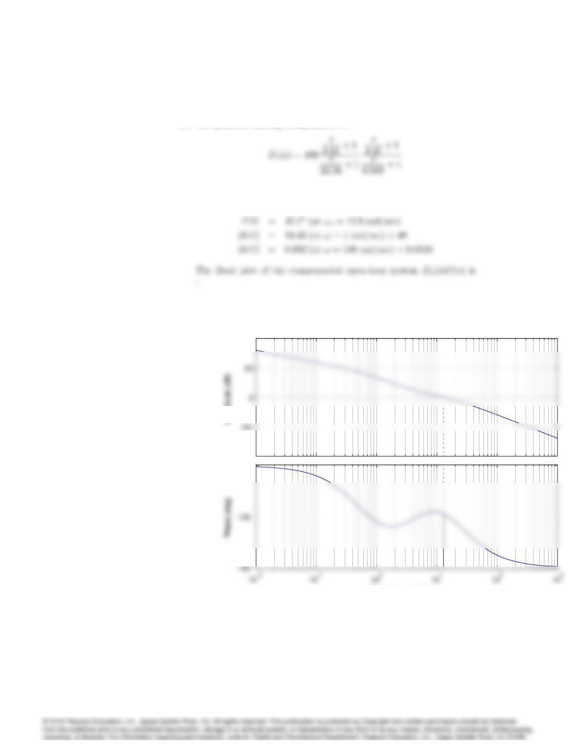
(f) One possible lead-lag compensator is :
which meets all the specification :
Kv= 100
–100
100
–90
Bode Diagram
Gm = Inf dB (at Inf rad/sec) , Pm = 47.7 deg (at 12.9 rad/sec)
Frequency (rad/sec)
–100
100
–90
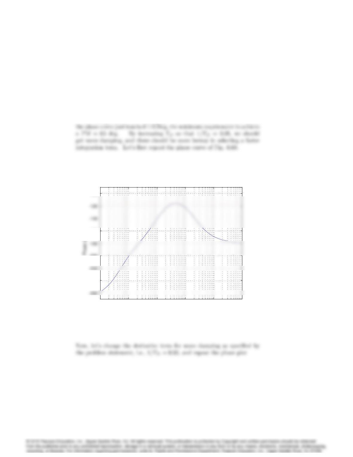
63. For Example 6.20, redo the design by selecting 1=TD= 0:05 and then
determining the highest possible value of 1=TIthat will meet the PM
6175
requirement. Then examine the improvement, if any, in the response to
a step disturbance torque.
Solution:
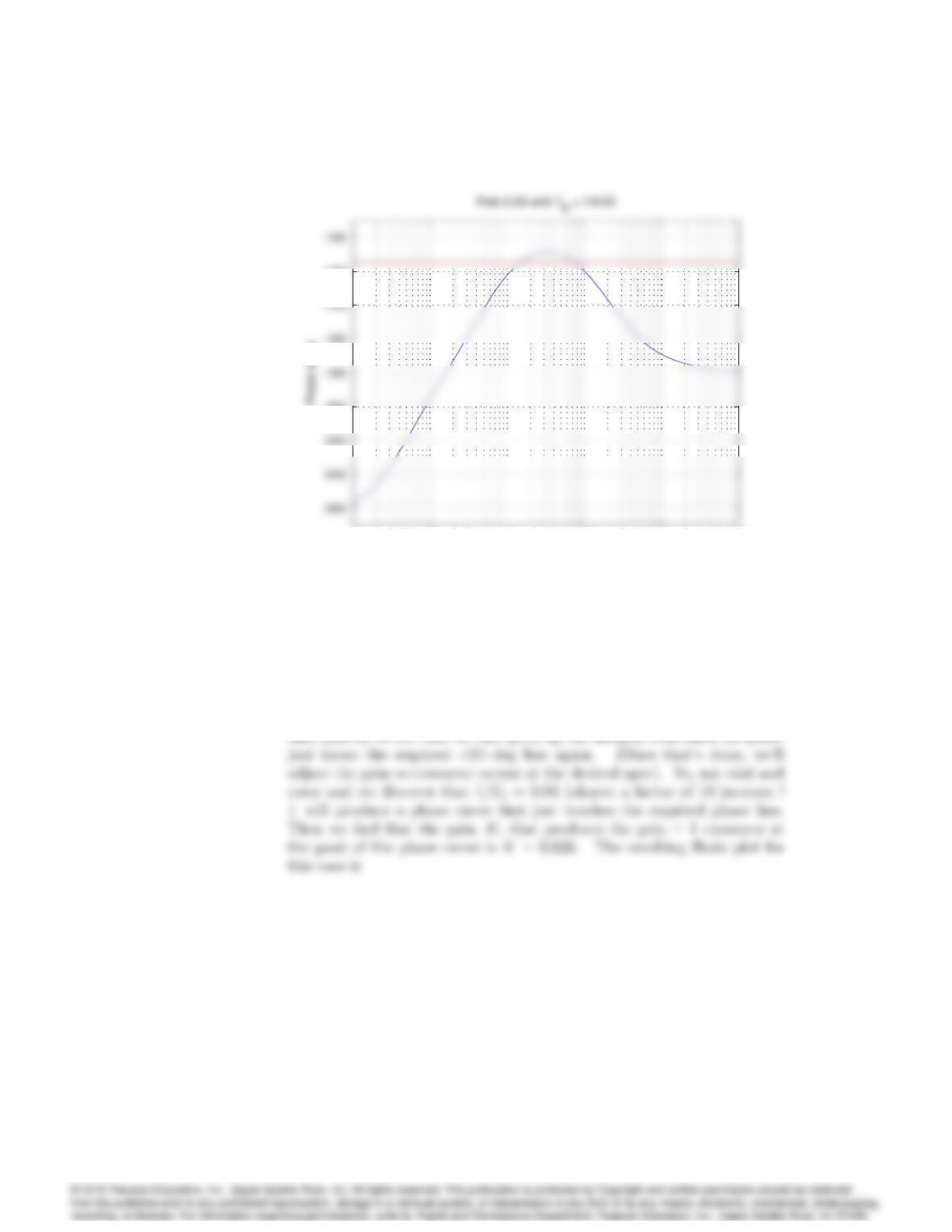
From Example 6:20, note that 1=TD= 0:1was selected for the case where
10-3 10-2 10-1 100101102
–240
–200
–160
–100
ω (rad/sec)
Prob 6.63, Ex 6.20 case
6176 CHAPTER 6. THE FREQUENCY-RESPONSE DESIGN METHOD
10-3 10-2 10-1 100101102
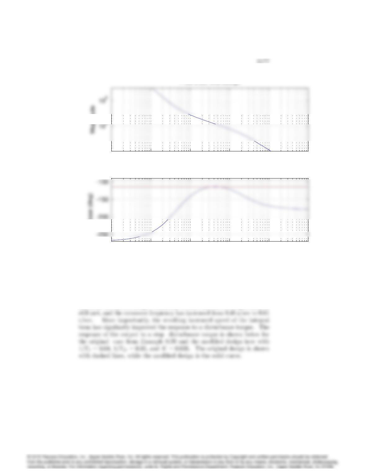
–200
–160
–120
ω (rad/sec)
10-3 10-2 10-1 100101102
10-2
ω (rad/sec)
Prob 6.63, final design
10-3 10-2 10-1 100101102
ω (rad/sec)
Phase (deg)
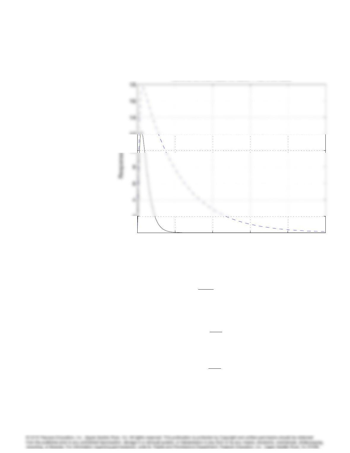
and from the Matlab margin command, we find that the PM requirement is
6178 CHAPTER 6. THE FREQUENCY-RESPONSE DESIGN METHOD
0200 400 600 800 1000
0
2
12
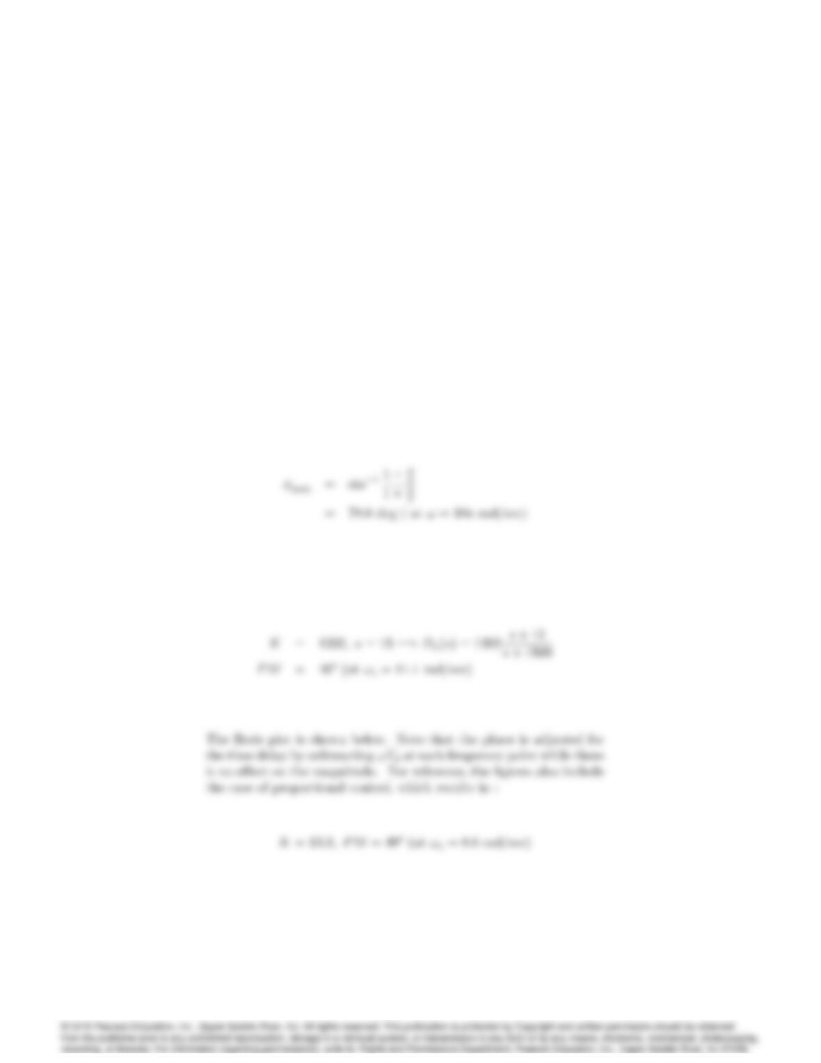
Nominal Ex 6:20 case vs faster Prob 6.63 case
Time (sec)
d
Problems and Solutions for Section 6.8
64. Assume that the system
G(s) = eTds
s+ 10;
has a 0.2-sec time delay (Td= 0:2sec). While maintaining a phase margin
40, find the maximum possible bandwidth using the following:
(a) One lead-compensator section
Dc(s) = Ks+a
s+b;
where b=a = 100;
(b) Two lead-compensator sections
Dc(s) = Ks+a
s+b2
;
where b=a = 10.
6179
(c) Comment on the statement in the text about the limitations on the
bandwidth imposed by a delay.
Solution :
(a) One lead section :
With b=a = 100, the lead compensator can add the maximum phase
lead :
By trial and error, a good compensator is :