6100 CHAPTER 6. THE FREQUENCY-RESPONSE DESIGN METHOD
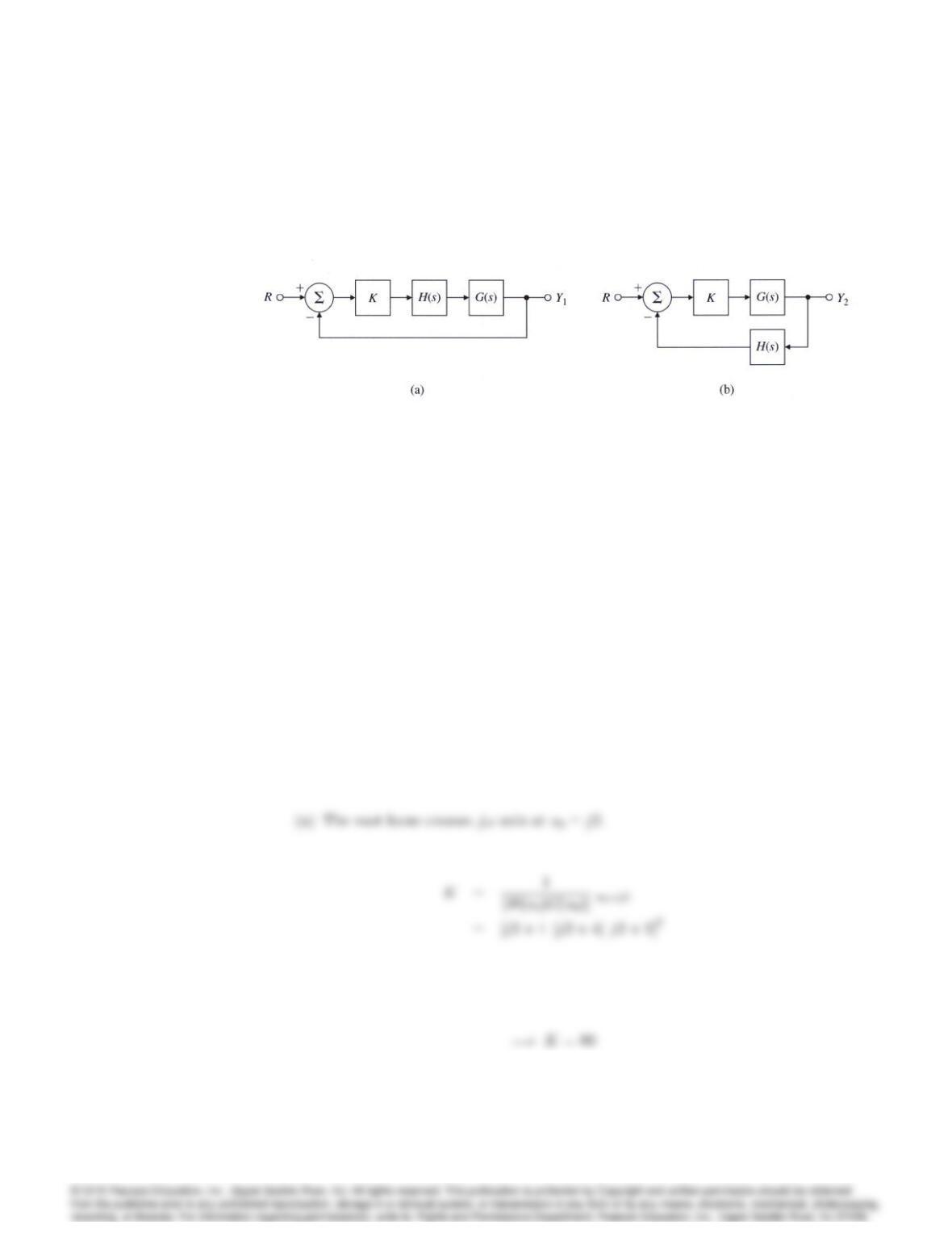
Figure 6.92: Block diagram for Problem 32: (a) unity feedback; (b) H(s)in
feedback
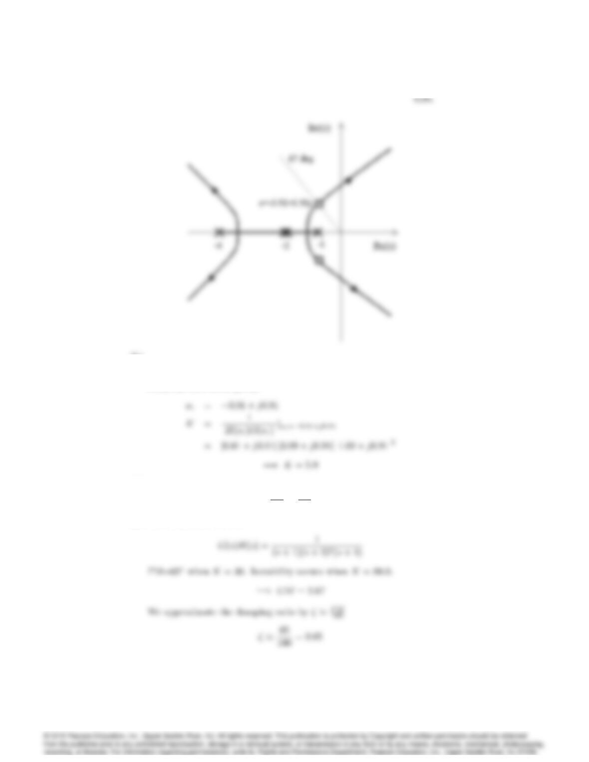
(e) Sketch a root locus for the system shown in Fig. 6.92(b).. How does
it differ from the one in part (a)?
(f) For the systems in Figs. 6.92(a) and (b), how does the transfer func-
tion Y2(s)=R(s)differ from Y1(s)=R(s)? Would you expect the step
response to r(t)be different for the two cases?
Solution :
(b)
= 0:707 =)0:707 = sin =)= 45
From the root locus given,
(c)
GM =Ka
Kb
=80
5:9= 13:5
(d) From the Root Locus :
6102 CHAPTER 6. THE FREQUENCY-RESPONSE DESIGN METHOD
10-2 10-1 100101102
10-10
Frequency (rad/sec)
Magnitude
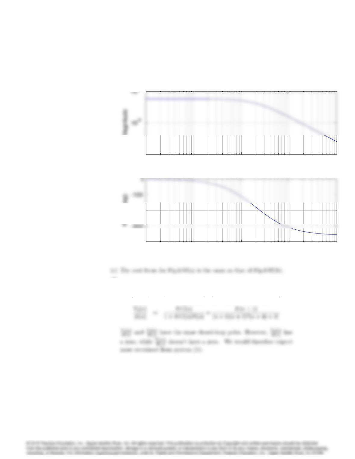
Bode plot for Prob. 6.32
10-2 10-1 100101102
10-10
Frequency (rad/sec)
Magnitude
Bode plot for Prob. 6.32
10-2 10-1 100101102
-400
-200
ω (rad/sec)
10-2 10-1 100101102
10-10
Frequency (rad/sec)
Magnitude
Bode plot for Prob. 6.32
10-2 10-1 100101102
10-10
Frequency (rad/sec)
Magnitude
Bode plot for Prob. 6.32
10-2 10-1 100101102
-400
-200
ω (rad/sec)
(f)
Y1(s)
R(s)=KG(s)H(s)
1 + KG(s)H(s)=K
(s+ 1)(s+ 2)2(s+ 4) + K
33. For the system shown in Fig. 6.93, use Bode and root-locus plots to deter-
mine the gain and frequency at which instability occurs. What gain (or
gains) gives a PM of 20? What is the GM when PM = 20?
Solution :
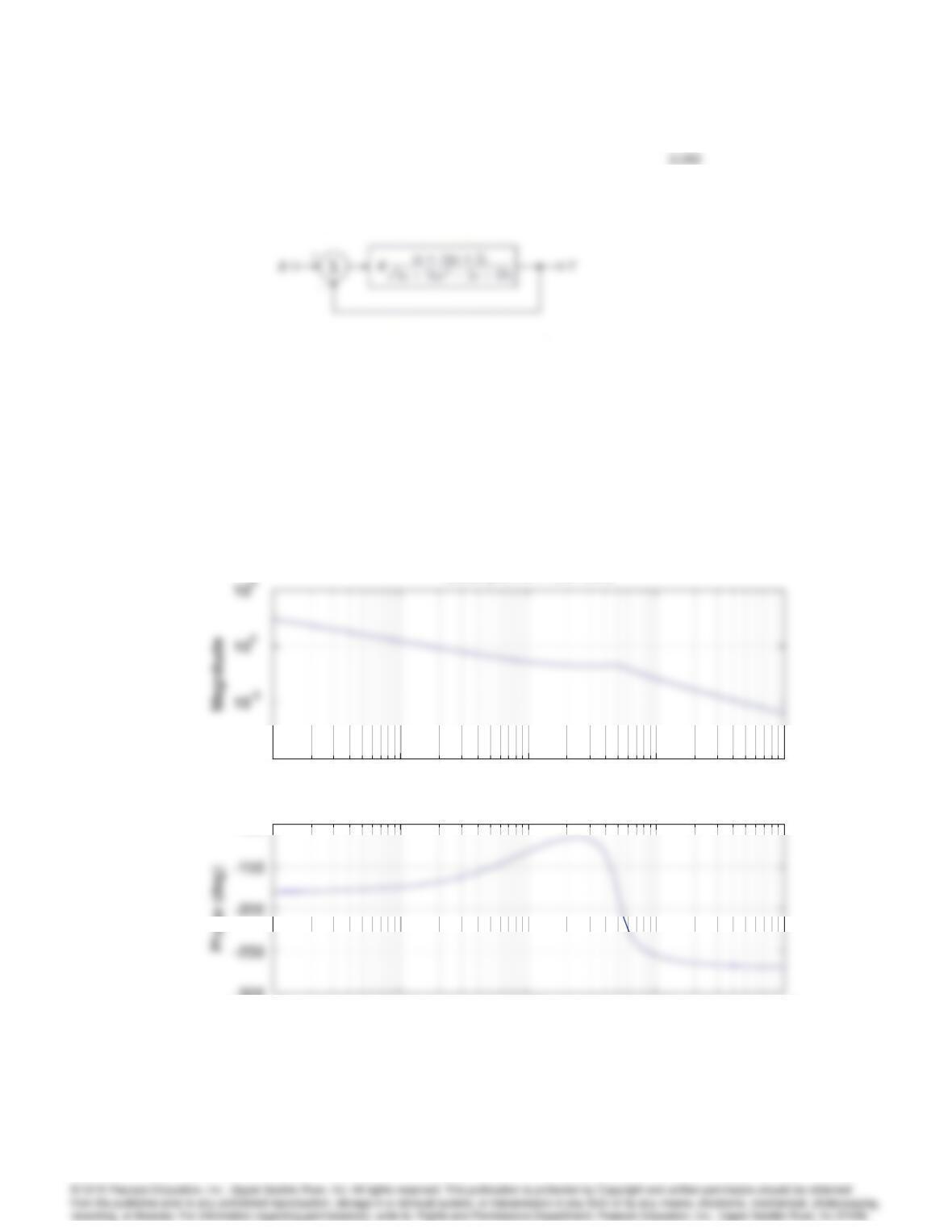
Figure 6.93: Control system for Problem 33
10-2 10-1 100101102
10-10
ω (rad/sec)
Bode plot for Prob. 6.33
10-2 10-1 100101102
10-10
ω (rad/sec)
Bode plot for Prob. 6.33
10-2 10-1 100101102
-300
-100
ω (rad/sec)
10-2 10-1 100101102
10-10
ω (rad/sec)
Bode plot for Prob. 6.33
10-2 10-1 100101102
10-10
ω (rad/sec)
Bode plot for Prob. 6.33
10-2 10-1 100101102
-300
-100
ω (rad/sec)
6104 CHAPTER 6. THE FREQUENCY-RESPONSE DESIGN METHOD
The system with K= 1 gives,
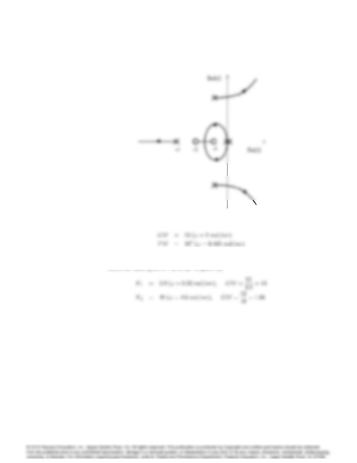
Therefore, instability occurs at K0= 52 and != 5 rad/sec.
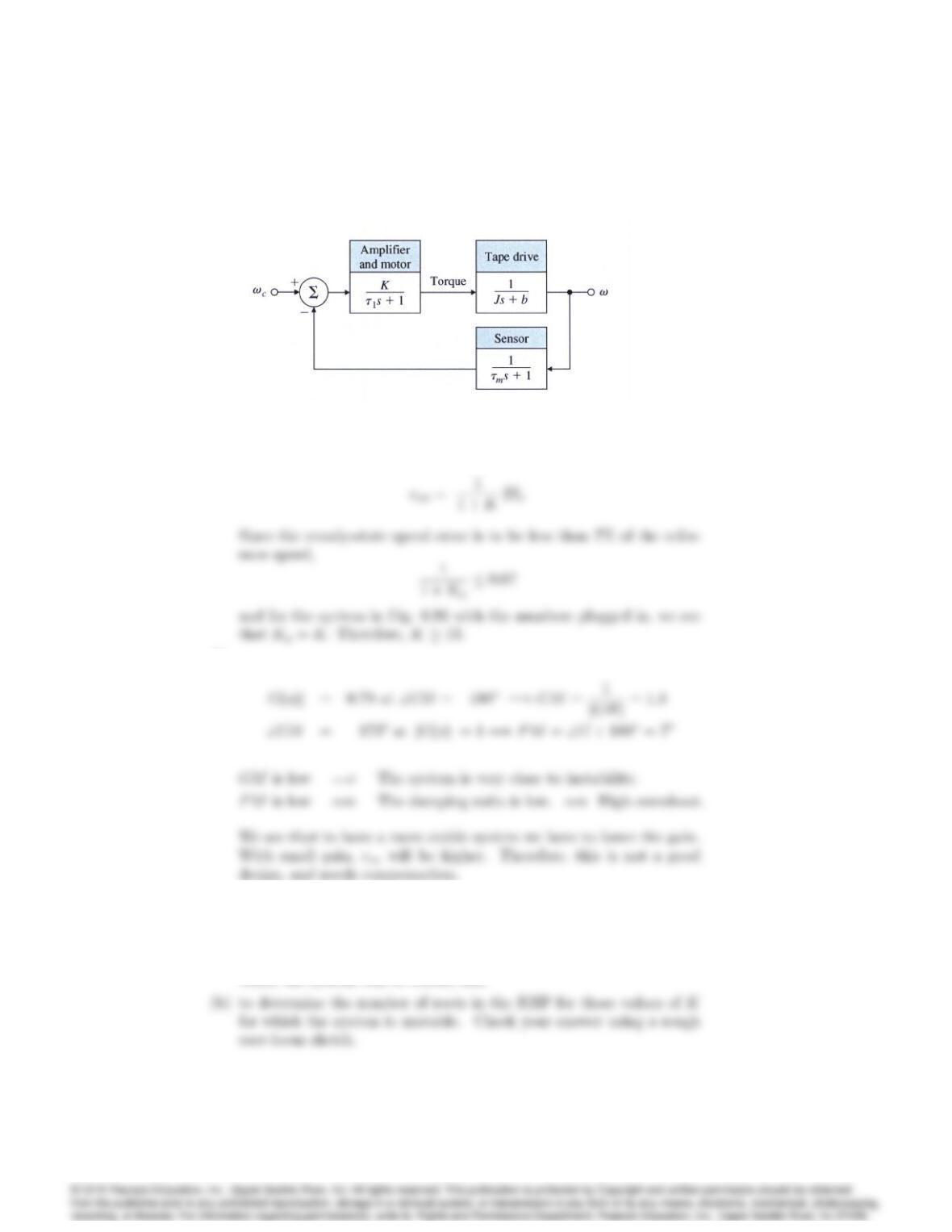
34. A magnetic tape-drive speed-control system is shown in Fig. 6.94. The
speed sensor is slow enough that its dynamics must be included. The
speed-measurement time constant is m= 0:5sec; the reel time constant
is r=J=b = 4 sec, where b= the output shaft damping constant =
1 N msec; and the motor time constant is 1= 1 sec.
(a) Determine the gain Krequired to keep the steady-state speed error
to less than 7% of the reference-speed setting.
(b) Determine the gain and phase margins of the system. Is this a good
system design?
Solution :
6105
Figure 6.94: Magnetic tape-drive speed control
(a) From Table 4.1, the error for this Type 1 system is
(b)
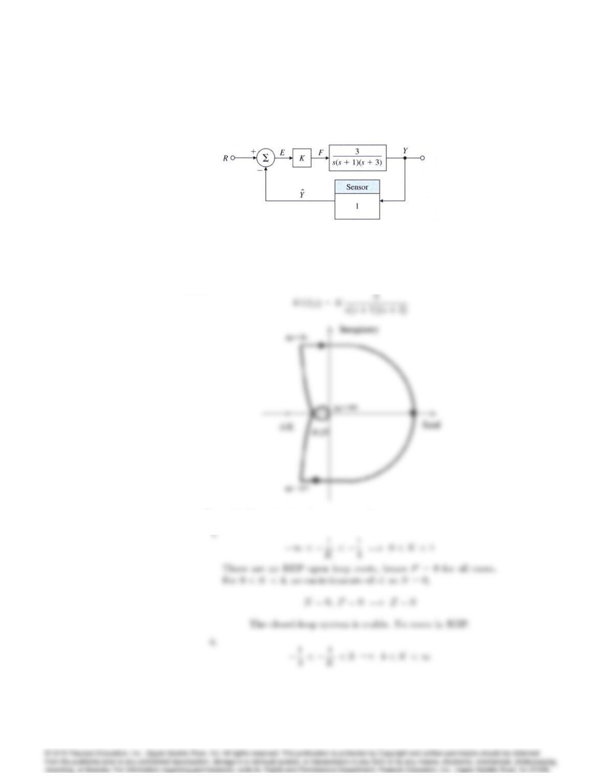
35. For the system in Fig. 6.95, determine the Nyquist plot and apply the
Nyquist criterion
(a) to determine the range of values of K(positive and negative) for
which the system will be stable, and
6106 CHAPTER 6. THE FREQUENCY-RESPONSE DESIGN METHOD
Figure 6.95: Control system for Problems 35, 69, and 70
Solution :
(a) & b.
From the Nyquist plot above, we see that:
6107
Two encirclements of the -1 point, hence
Two closed-loop roots in RHP.
iii.
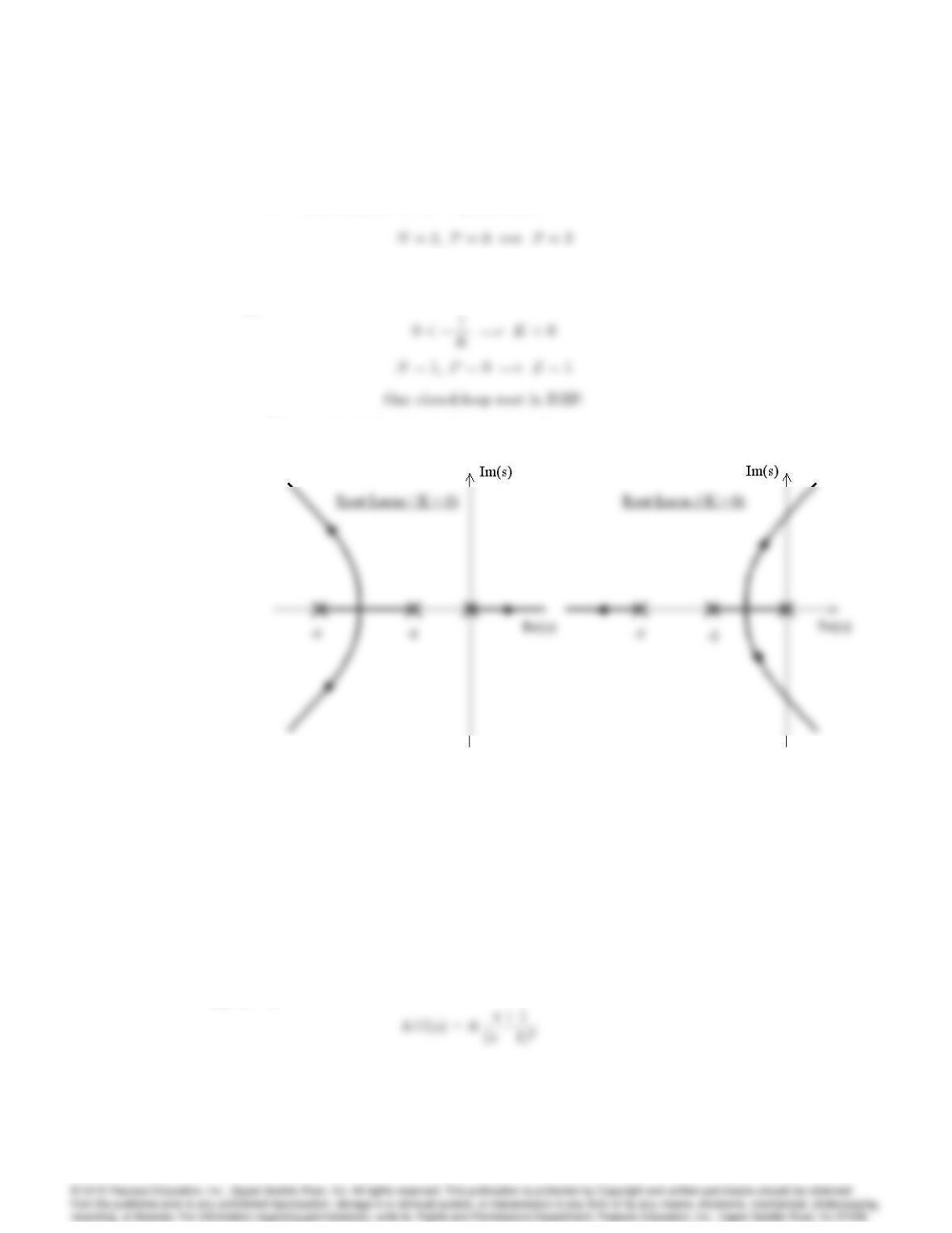
The root loci below show the same results.
36. For the system shown in Fig. 6.96, determine the Nyquist plot and apply
the Nyquist criterion.
(a) to determine the range of values of K(positive and negative) for
which the system will be stable, and
(b) to determine the number of roots in the RHP for those values of K
for which the system is unstable. Check your answer using a rough
root-locus sketch.
Solution :
(a) & b.
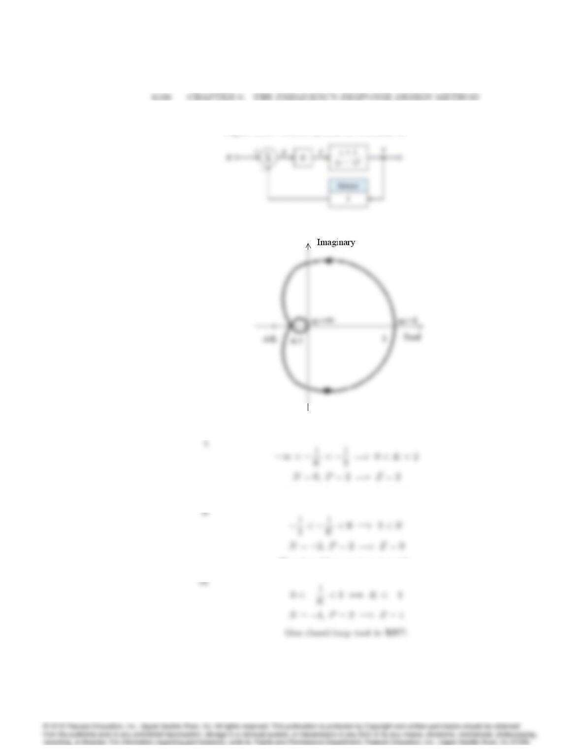
Figure 6.96: Control system for Problem 36
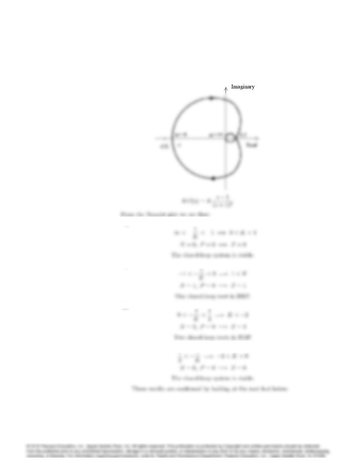
From the Nyquist plot we see that:
Two closed-loop roots in RHP.
The closed-loop system is stable.
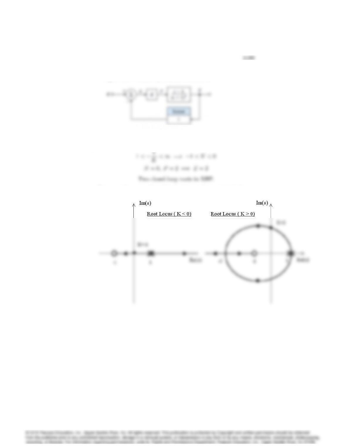
Figure 6.97: Control system for Problem 37
iv.
These results are con…rmed by looking at the root loci below:
37. For the system shown in Fig. 6.97, determine the Nyquist plot and apply
the Nyquist criterion.
(a) to determine the range of values of K(positive and negative) for
which the system will be stable, and
(b) to determine the number of roots in the RHP for those values of K
for which the system is unstable. Check your answer using a rough
root-locus sketch.
Solution :
6110 CHAPTER 6. THE FREQUENCY-RESPONSE DESIGN METHOD
(a) & b.
ii.
iv. 1
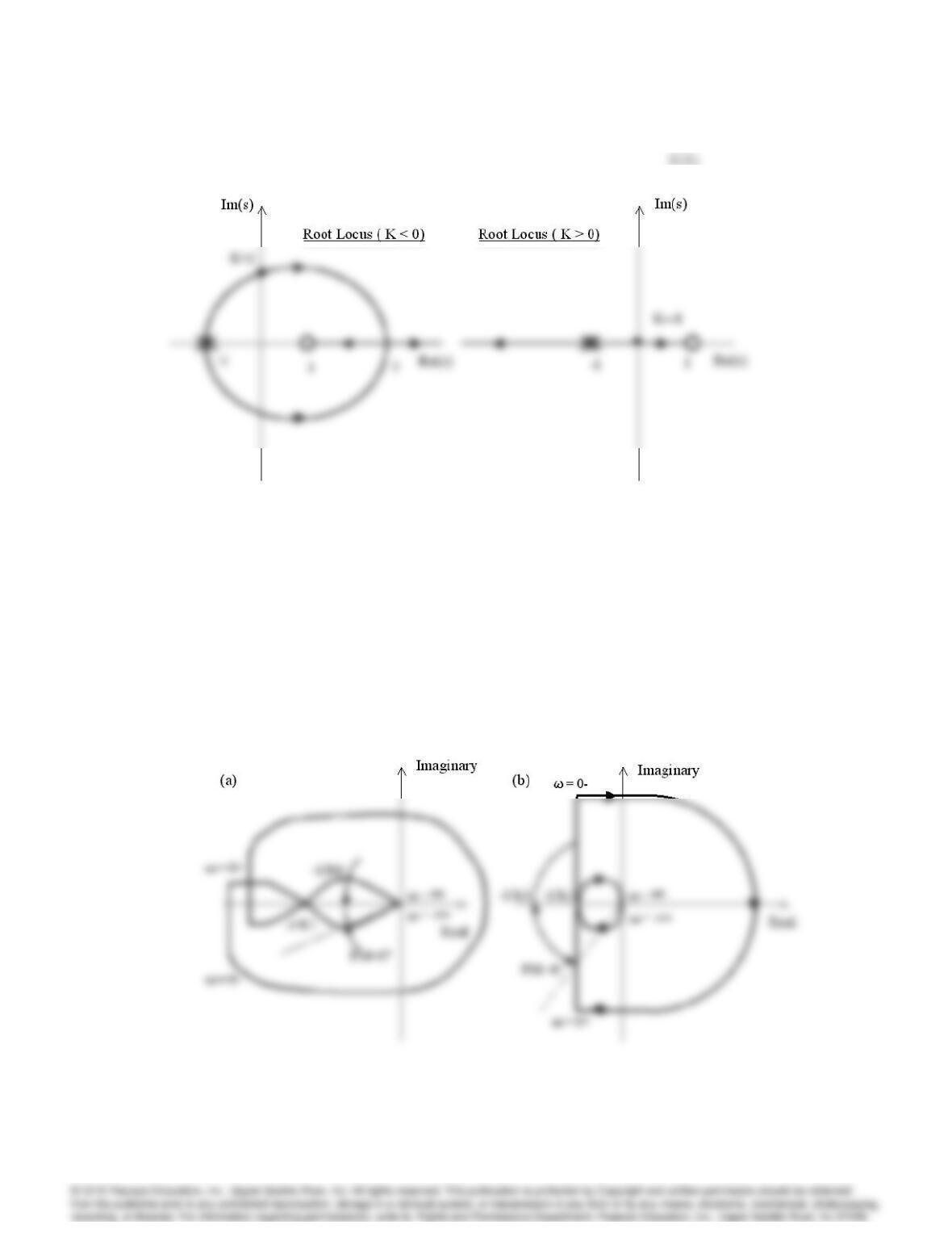
38. The Nyquist diagrams for two stable, open-loop systems are sketched in
Fig. 6.98. The proposed operating gain is indicated as K0, and arrows
indicate increasing frequency. In each case give a rough estimate of the
following quantities for the closed-loop (unity feedback) system:
(a) phase margin
(b) damping ratio
(c) range of gain for stability (if any)
(d) system type (0, 1, or 2).
Solution :
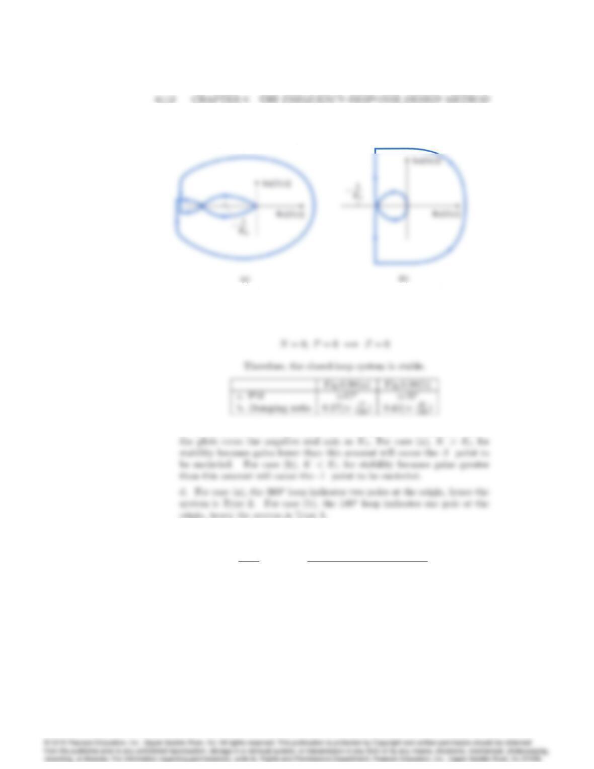
Figure 6.98: Nyquist plots for Problem 38
For both, with K=K0:
c. To determine the range of gain for stability, call the value of Kwhere
39. The steering dynamics of a ship are represented by the transfer function
V(s)
r(s)=G(s) = K[(s=0:142) + 1]
s(s=0:325 + 1)(s=0:0362 + 1);
where vis the ship’s lateral velocity in meters per second, and ris the
rudder angle in radians.
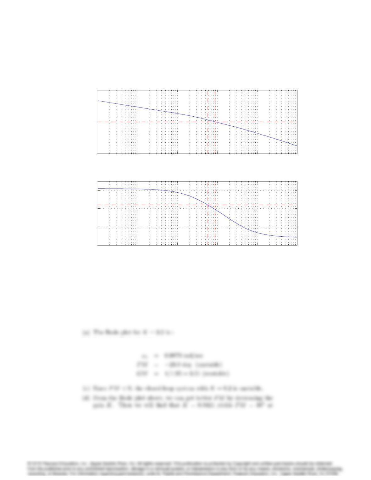
(a) Use the MATLAB command bode to plot the log magnitude and
phase of G(j!)for K= 0:2
(b) On your plot, indicate the crossover frequency, PM, and GM,
6113
10-4 10-3 10-2 10-1 100101
10-5
100
105
ω (rad/sec)
Magnitude
Bode plot for Prob 6.39, K=0.2
10-4 10-3 10-2 10-1 100101
-400
-300
-200
-100
ω (rad/sec)
Phase (deg)
(c) Is the ship steering system stable with K= 0:2?
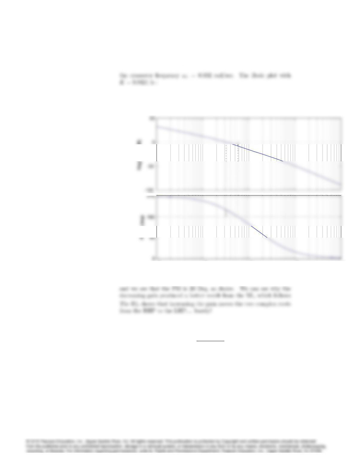
(d) What value of Kwould yield a PM of 30oand what would the
crossover frequency be?
Solution :
(b) From the Bode plot above :
6114 CHAPTER 6. THE FREQUENCY-RESPONSE DESIGN METHOD
10
-3
10
-2
10
-1
10
0
10
1
Bode Diagram
Gm = 7.68 dB (at 0.0576 rad/sec) , Pm = 30 deg (at 0.0321 rad/sec)
Frequency (rad/sec)
10
-3
10
-2
10
-1
10
0
10
1
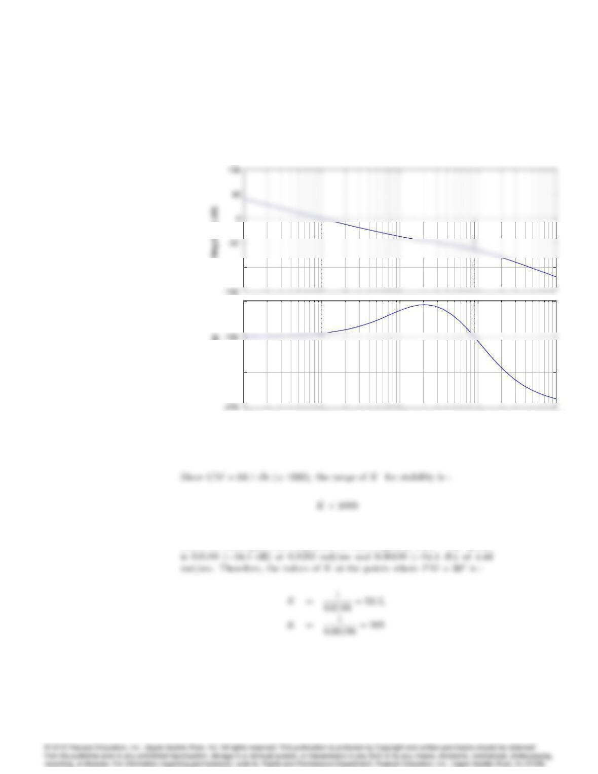
40. For the open-loop system
KG(s) = K(s+ 1)
s2(s+ 10)2:
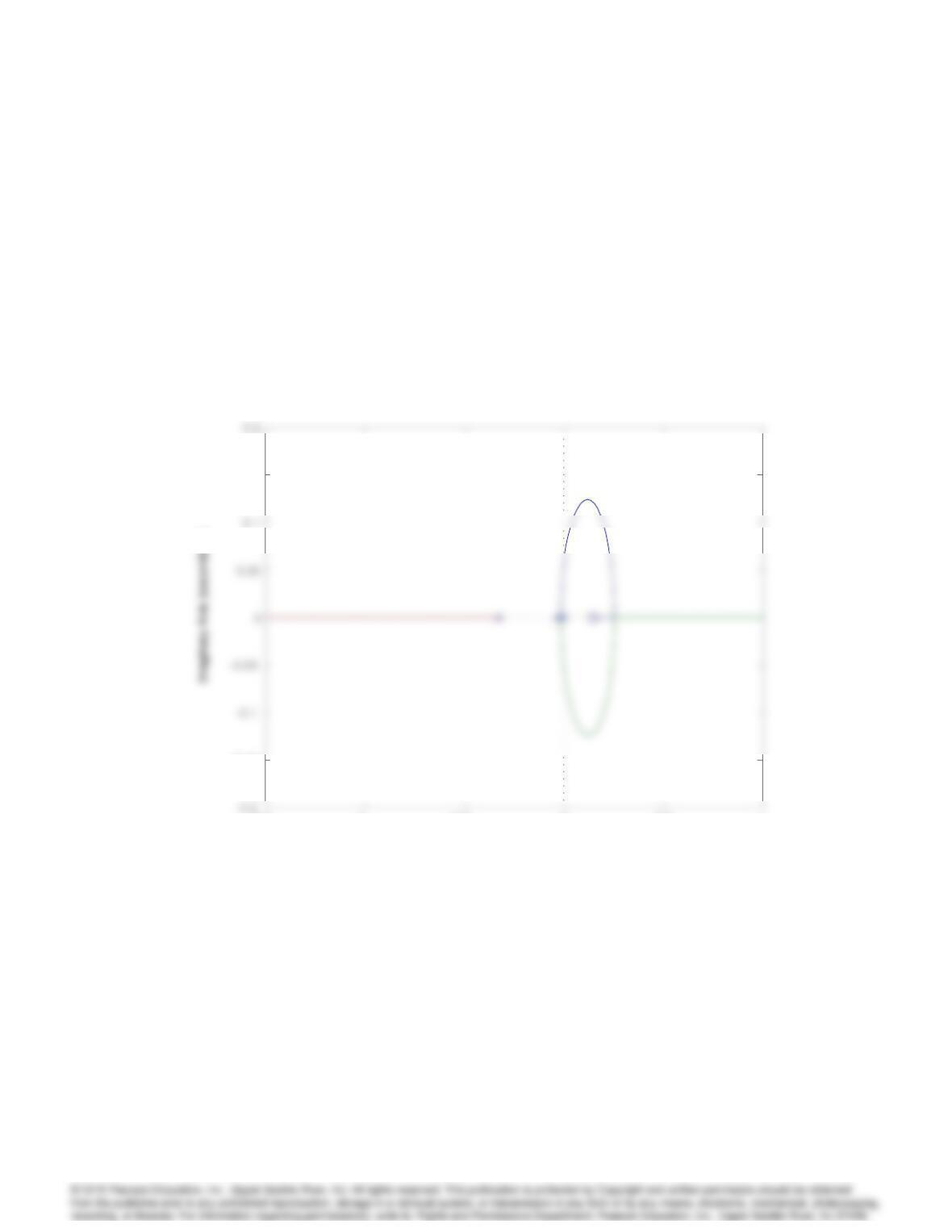
Determine the value for Kat the stability boundary and the values of K
at the points where P M = 30.
Solution :
The bode plot of this system with K= 1 is :
6115
–1.5 -1 -0.5 00.5 1
–0.15
0.15
Root Locus
Real Axis (seconds
-1
)
-1
)
6116 CHAPTER 6. THE FREQUENCY-RESPONSE DESIGN METHOD
–100
10
-2
10
-1
10
0
10
1
10
2
–225
–135
Phase (deg)
Bode Diagram
Gm = 64.1 dB (at 8.94 rad/sec) , Pm = 4.58 deg (at 0.1 rad/sec)
Frequency (rad/sec)
–100
10
-2
10
-1
10
0
10
1
10
2
–225
–135
Phase (deg)
From the Bode plot, the magnitude at the frequency with 150phase
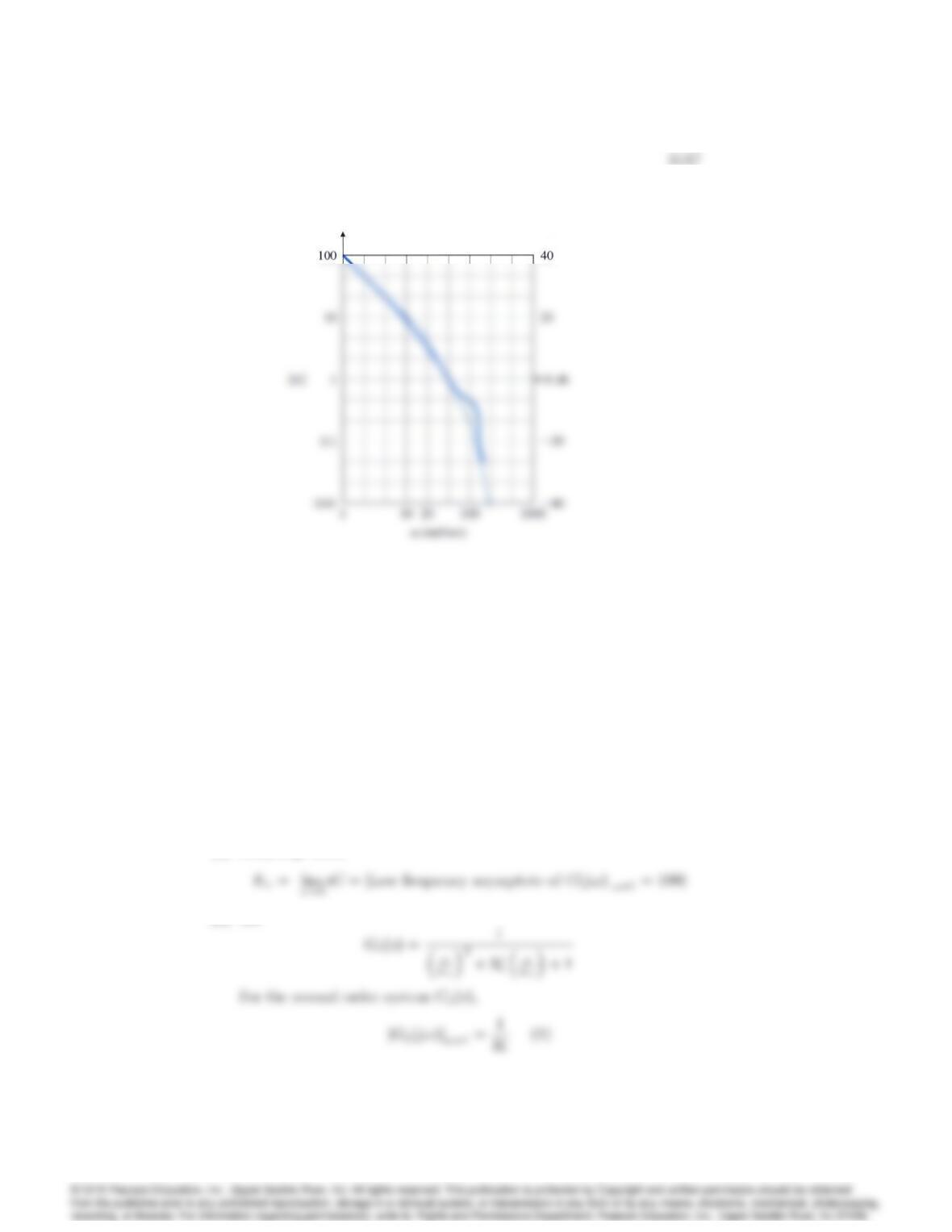
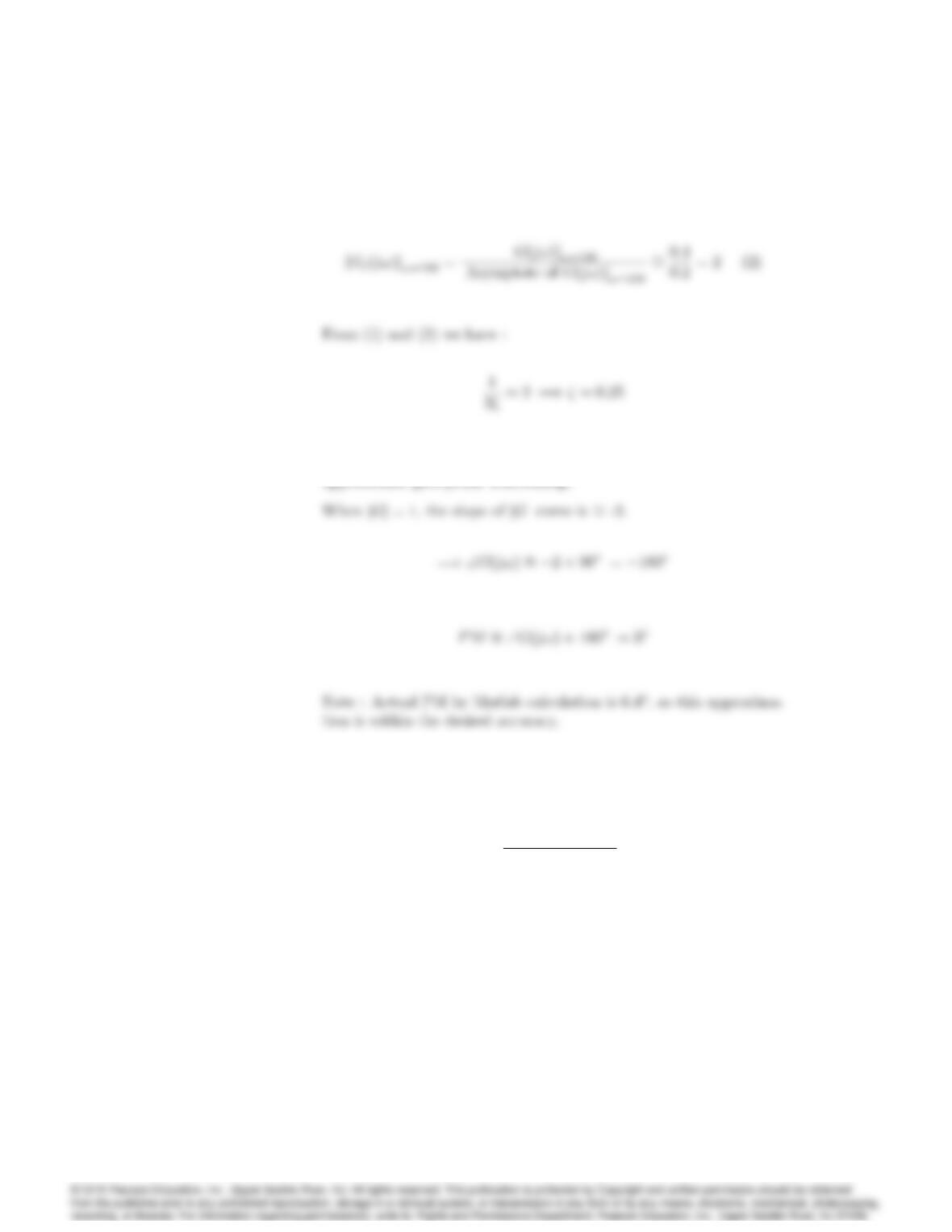
Figure 6.99: Magnitude frequency response for Problem 41
(a) Problems and Solutions for Section 6.5
41. The frequency response of a plant in a unity feedback con…guration is
sketched in Fig. 6.99. Assume the plant is open-loop stable and minimum
phase.
(a) What is the velocity constant Kvfor the system as drawn?
(b) What is the damping ratio of the complex poles at != 100?
(c) What is the PM of the system as drawn? (Estimate to within 10o.)
Solution :
(a) From Fig. 6.99,
(b) Let
6118 CHAPTER 6. THE FREQUENCY-RESPONSE DESIGN METHOD
From Fig. 6.99 :
(c) Since the plant is a minimum phase system, we can apply the Bode’s
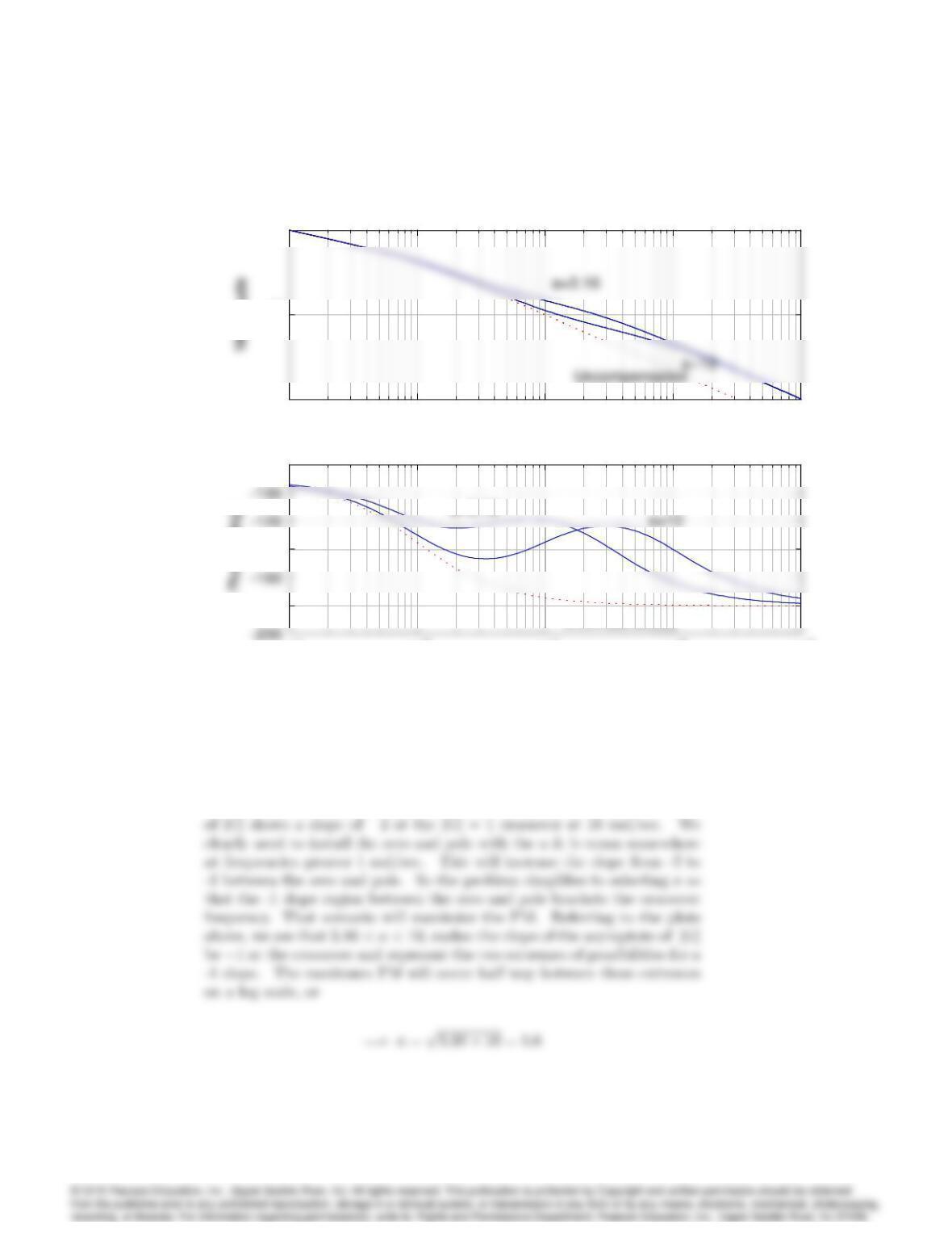
42. For the system
G(s) = 100(s=a + 1)
s(s+ 1)(s=b + 1);
where b= 10a, …nd the approximate value of athat will yield the best PM
by sketching only candidate values of the frequency response magnitude.
Solution :
6119
10-1 100101102103
100
Frequency (rad/sec)
Bode Diagrams
10-1 100101102103
-180
-140
-80
ω (rad/sec)
10-1 100101102103
100
Frequency (rad/sec)
Bode Diagrams
10-1 100101102103
100
Frequency (rad/sec)
Bode Diagrams
10-1 100101102103
-180
-140
-80
ω (rad/sec)
a=3.16 a=10
Uncompensated
10-1 100101102103
100
Frequency (rad/sec)
Bode Diagrams
Without the zero and pole that contain the a & b terms, the plot