
6000
Solutions Manual: Chapter 6
7th Edition
Feedback Control of Dynamic
Systems
Gene F. Franklin
J. David Powell
Abbas Emami-Naeini
.Assisted by:
H. K. Aghajan
H. Al-Rahmani
P. Coulot
P. Dankoski
S. Everett
R. Fuller
T. Iwata
V. Jones
F. Safai
L. Kobayashi
H-T. Lee
E. Thuriyasena
M. Matsuoka
Chapter 6
The Frequency-response
Design Method
Problems and Solutions for Section 6.1
1. (a) Show that 0in Eq. (6.2) is given by
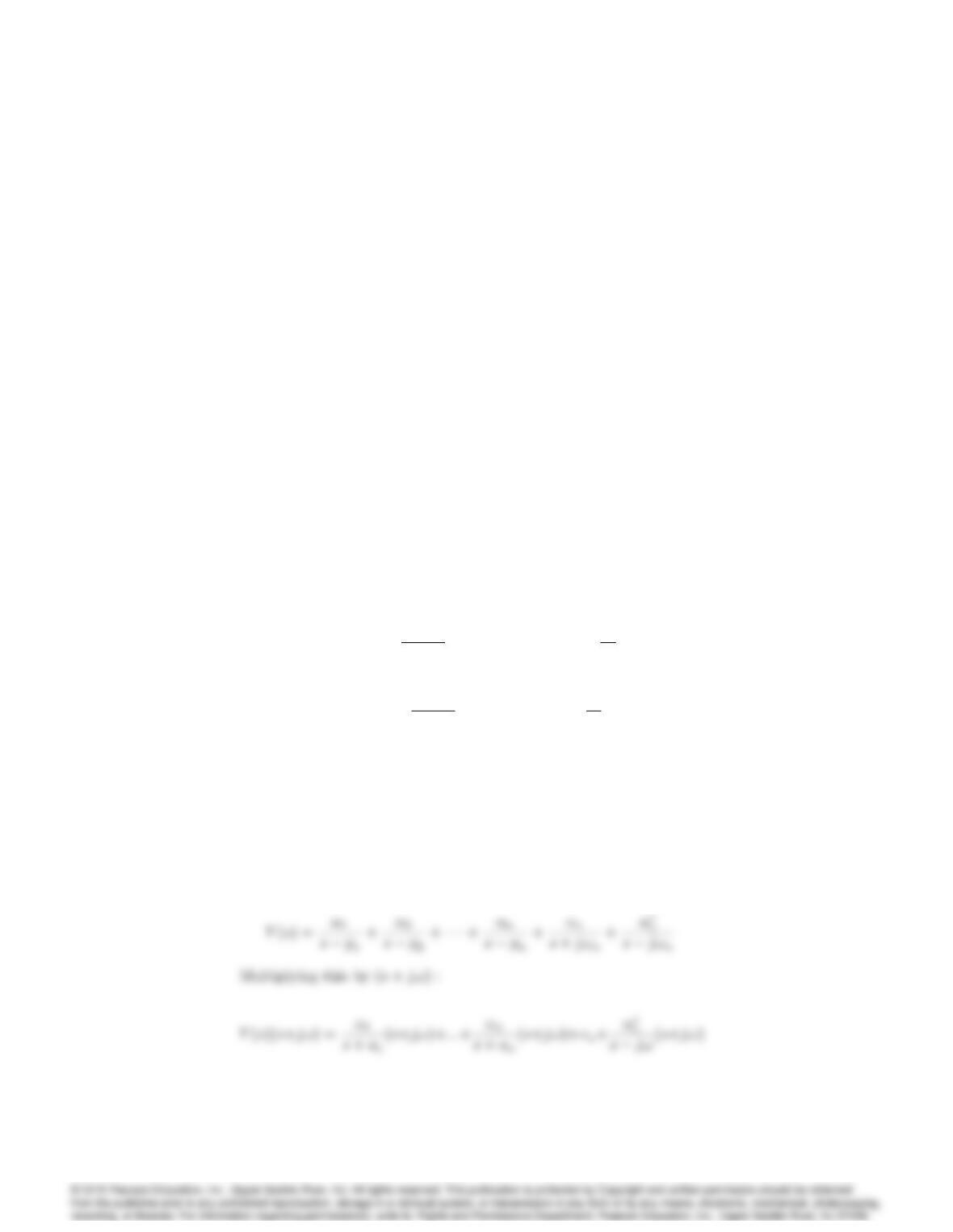
0=G(s)U0!
sj! s=j!
=U0G(j!)1
2j
and
0=G(s)U0!
s+j! s=+j!
=U0G(j!)1
2j:
(b) By assuming the output can be written as
y(t) = 0ej!t +
0ej!t;
derive Eqs. (6.4) – (6.6).
Solution:
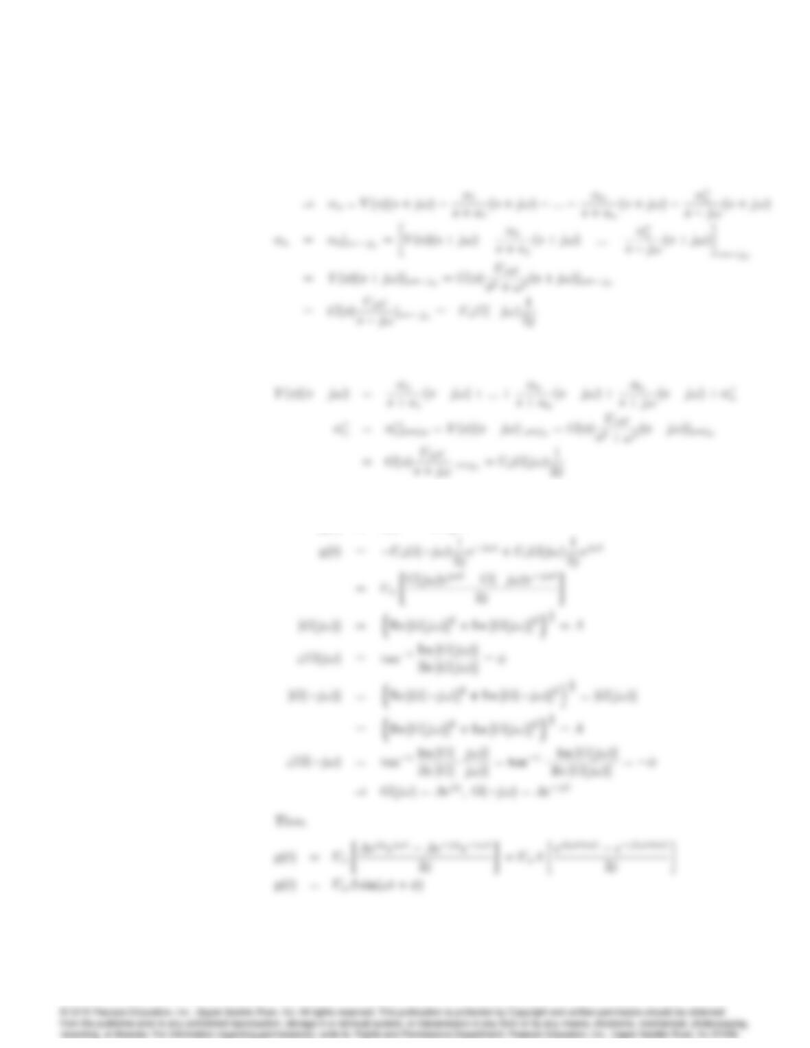
(a) Eq. (6.2):
6001
6002 CHAPTER 6. THE FREQUENCY-RESPONSE DESIGN METHOD
Similarly, multiplying Eq. (6.2) by (sj!):
(b)
y(t) = oej!t +
oej!t
2. (a) Calculate the magnitude and phase of
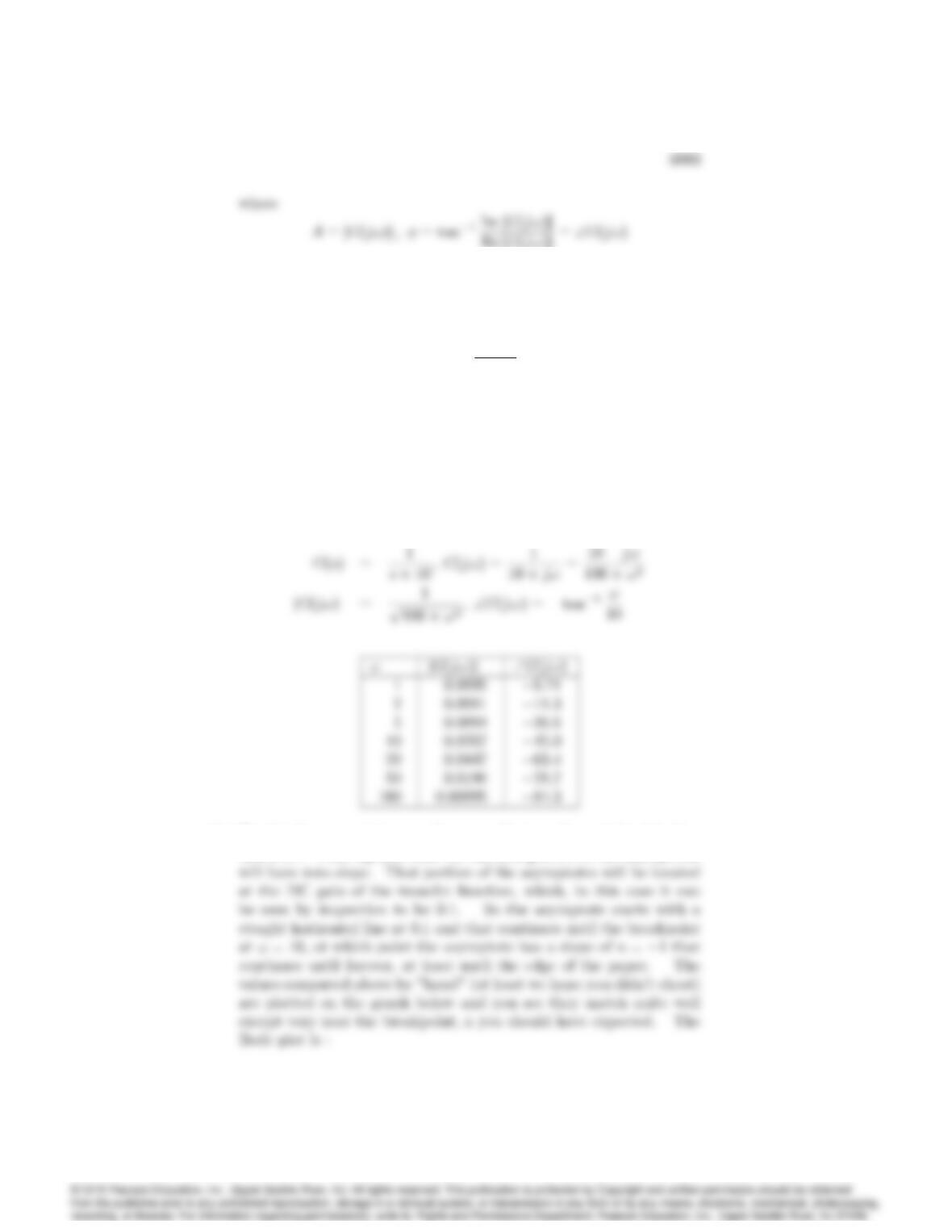
G(s) = 1
s+ 10
by hand for != 1, 2, 5, 10, 20, 50, and 100 rad/sec.
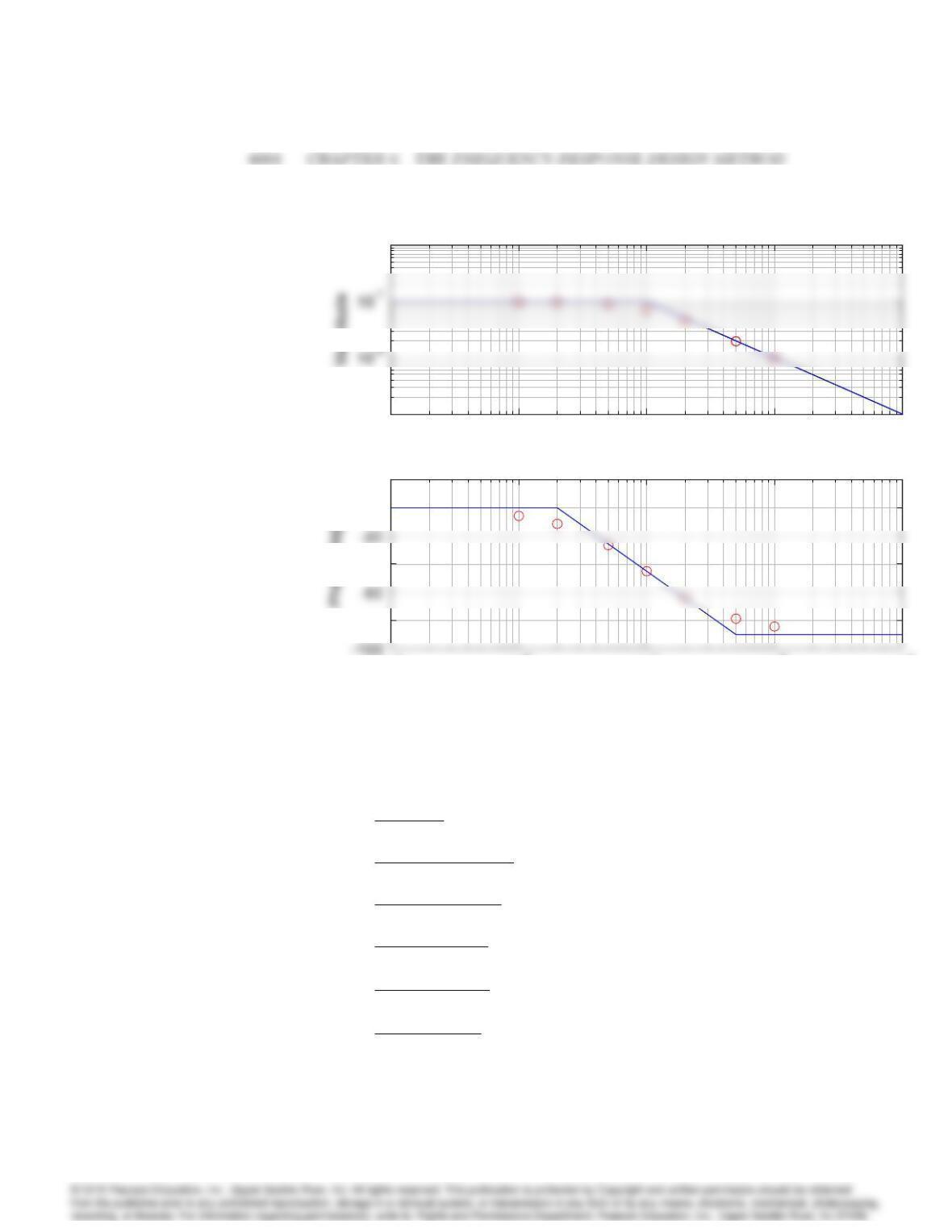
(b) sketch the asymptotes for G(s)according to the Bode plot rules, and
compare these with your computed results from part (a).
Solution:
(a)
(b) To plot the asymptotes, you first note that n= 0;as defined in Sec-
tion 6.1.1. That signifies that the leftmost portion of the asymptotes
10-1 100101102103
10-3
100
ω (rad/sec)
Bode plot for Problem 6.2
10-1 100101102103
10-3
100
ω (rad/sec)
Bode plot for Problem 6.2
10-1 100101102103
-80
-40
0
20
ω (rad/sec)
10-1 100101102103
10-3
100
ω (rad/sec)
Bode plot for Problem 6.2
10-1 100101102103
10-3
100
ω (rad/sec)
Bode plot for Problem 6.2
10-1 100101102103
-80
-40
0
20
ω (rad/sec)
3. Sketch the asymptotes of the Bode plot magnitude and phase for each
of the following open-loop transfer functions. After completing the hand
sketches verify your result using MATLAB. Turn in your hand sketches
and the MATLAB results on the same scales.
(a) L(s) = 2000
s(s+ 200)
(b) L(s) = 100
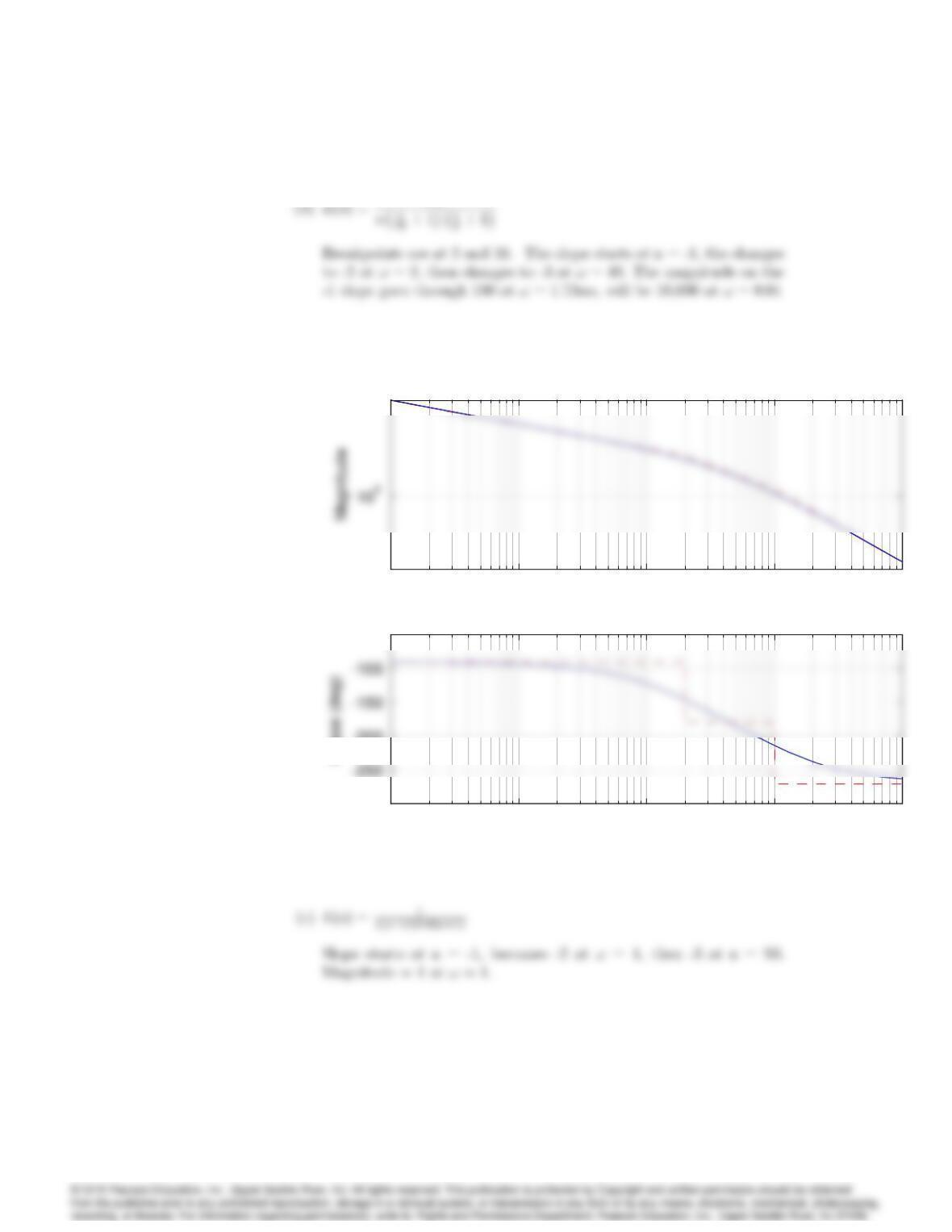
s(0:1s+ 1)(0:5s+ 1)
(c) L(s) = 1
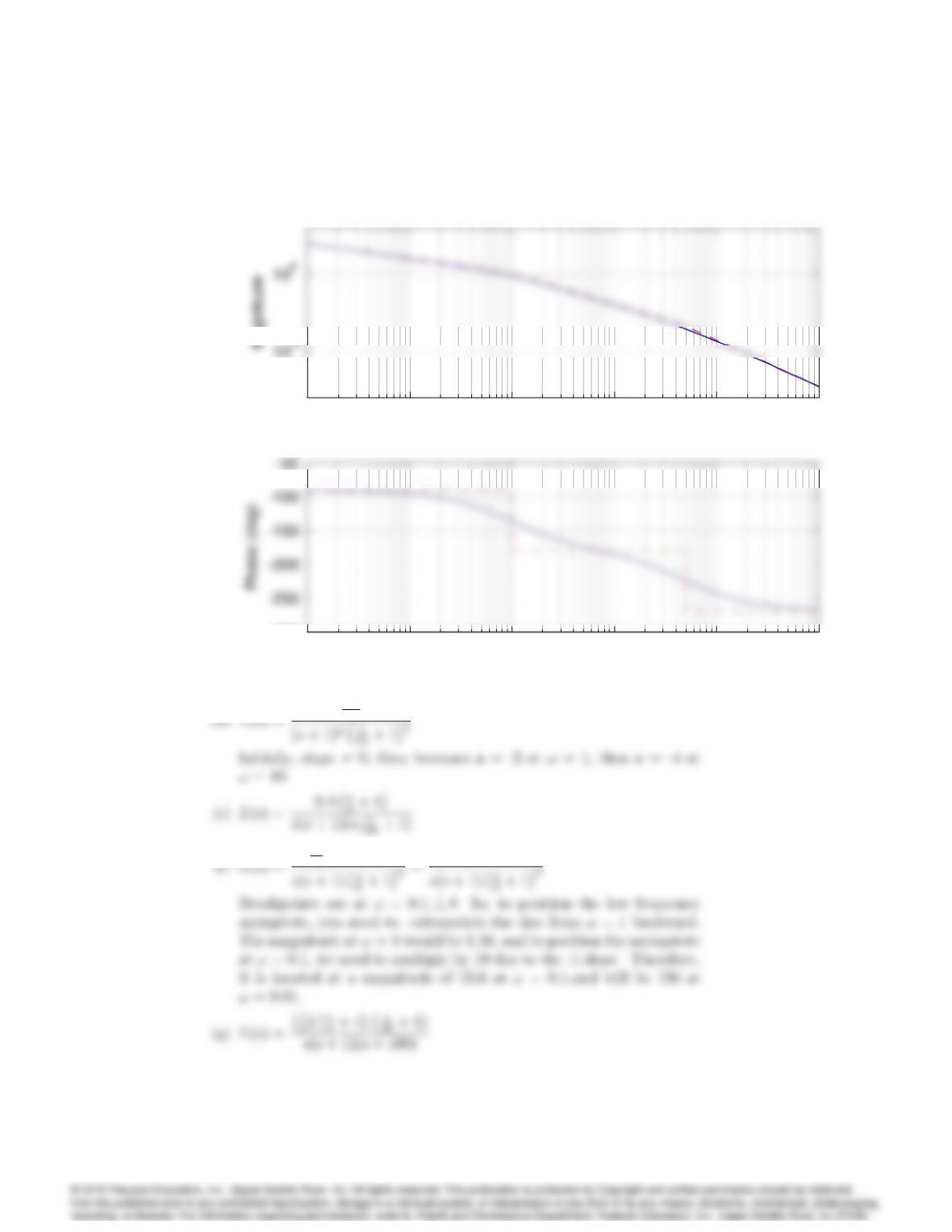
s(s+ 1)(0:02s+ 1)
(d) L(s) = 1
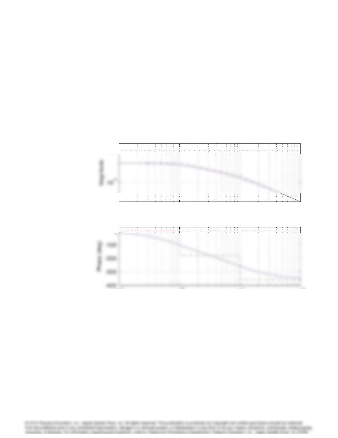
(s+ 1)2(s+ 10)2
(e) L(s) = 10(s+ 4)
s(s+ 1)(s+ 100)
(f) L(s) = 1000(s+ 0:1)
s(s+ 1)(s+ 8)2
6005
(g) L(s) = (s+ 5)(s+ 10)
s(s+ 1)(s+ 100)
(h) L(s) = 4s(s+ 10)
(s+ 100)(s+ 500)
(i) L(s) = s
(s+ 1)(s+ 10)(s+ 50)
Solution:
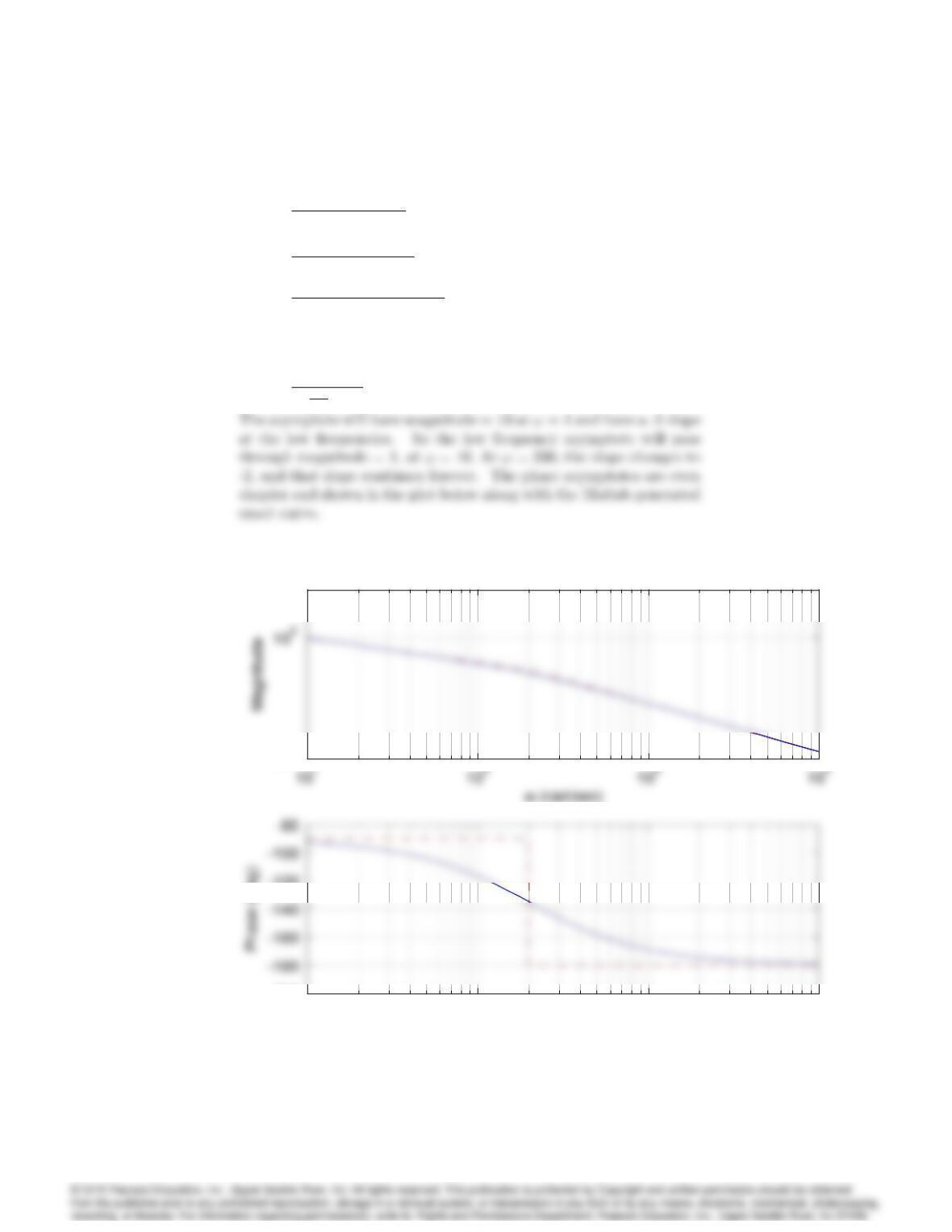
(a) L(s) = 10
ss
200 + 1
10-5
Bode plot for Prob. 6.3 (a)
10-5
Bode plot for Prob. 6.3 (a)
101102103104
-200
-120
ω (rad/sec)
10-5
Bode plot for Prob. 6.3 (a)
10-5
Bode plot for Prob. 6.3 (a)
101102103104
-200
-120
ω (rad/sec)
6006 CHAPTER 6. THE FREQUENCY-RESPONSE DESIGN METHOD
10-2 10-1 100101102
ω (rad/sec)
Bode plot for Prob. 6.3 (b)
10-2 10-1 100101102
ω (rad/sec)
Bode plot for Prob. 6.3 (b)
10-2 10-1 100101102
-300
-200
-50
ω (rad/sec)
Phase (deg)
10-2 10-1 100101102
ω (rad/sec)
Bode plot for Prob. 6.3 (b)
10-2 10-1 100101102
ω (rad/sec)
Bode plot for Prob. 6.3 (b)
10-2 10-1 100101102
-300
-200
-50
ω (rad/sec)
Phase (deg)
6007
10-2 10-1 100101102103
ω (rad/sec)
Bode plot for Prob. 6.3 (c)
10-2 10-1 100101102103
ω (rad/sec)
Bode plot for Prob. 6.3 (c)
10-2 10-1 100101102103
-300
ω (rad/sec)
10-2 10-1 100101102103
ω (rad/sec)
Bode plot for Prob. 6.3 (c)
10-2 10-1 100101102103
ω (rad/sec)
Bode plot for Prob. 6.3 (c)
10-2 10-1 100101102103
-300
ω (rad/sec)
1
100
32 (10s+ 1)
6008 CHAPTER 6. THE FREQUENCY-RESPONSE DESIGN METHOD
10-1 100101102
100
ω (rad/sec)
Bode plot for Prob 6.3(d)
10-1 100101102
ω (rad/sec)
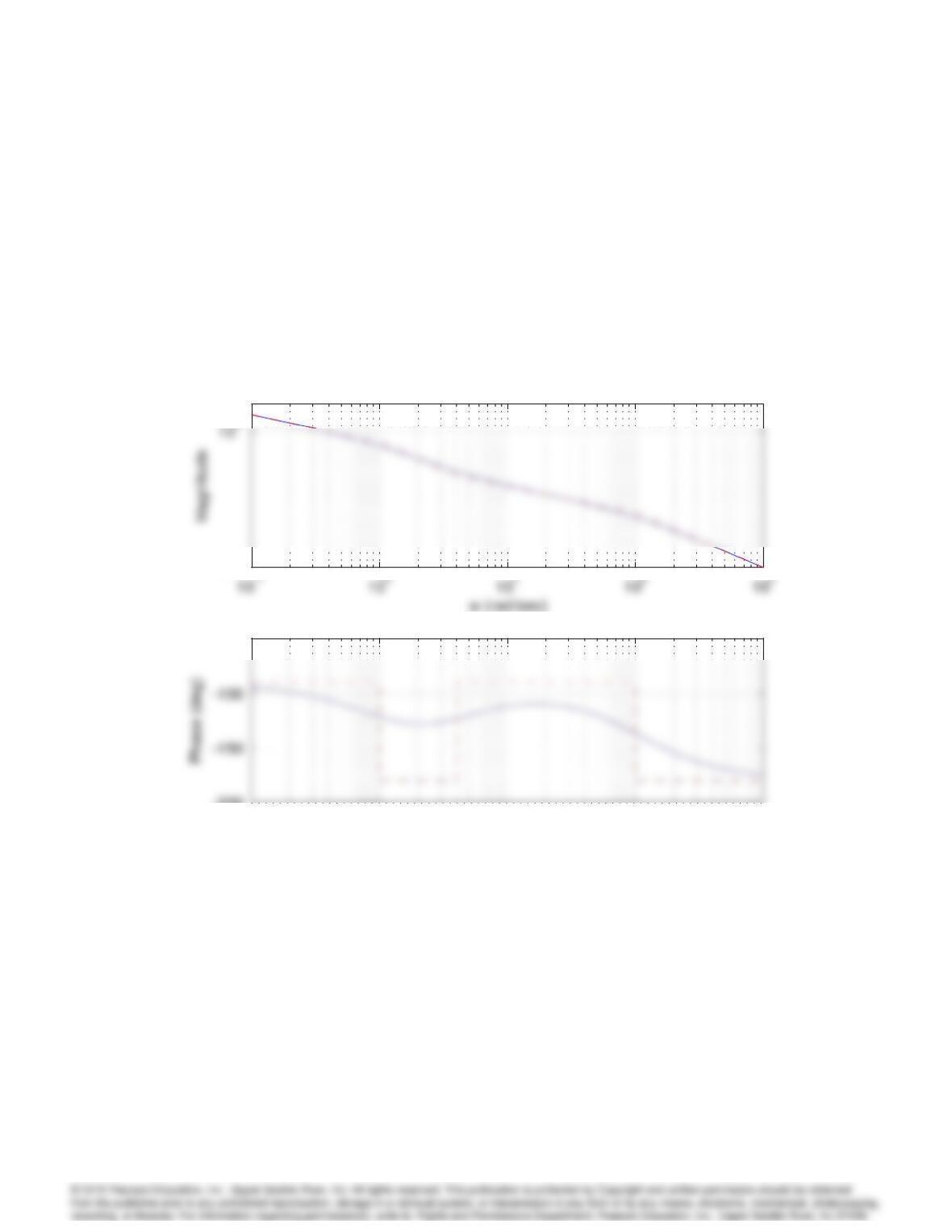
6009
10-5
Bode plot for Prob 6.3(e)
10-1 100101102103
-200
-50
ω (rad/sec)
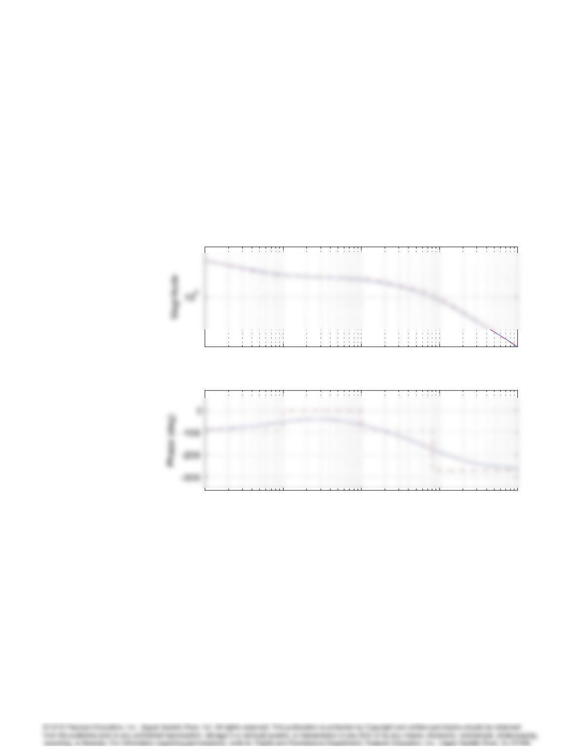
6010 CHAPTER 6. THE FREQUENCY-RESPONSE DESIGN METHOD
10-2 10-1 100101102
ω(rad/sec)
Bode plot for Prob 6.3(f)
10-2 10-1 100101102
ω (rad/sec)
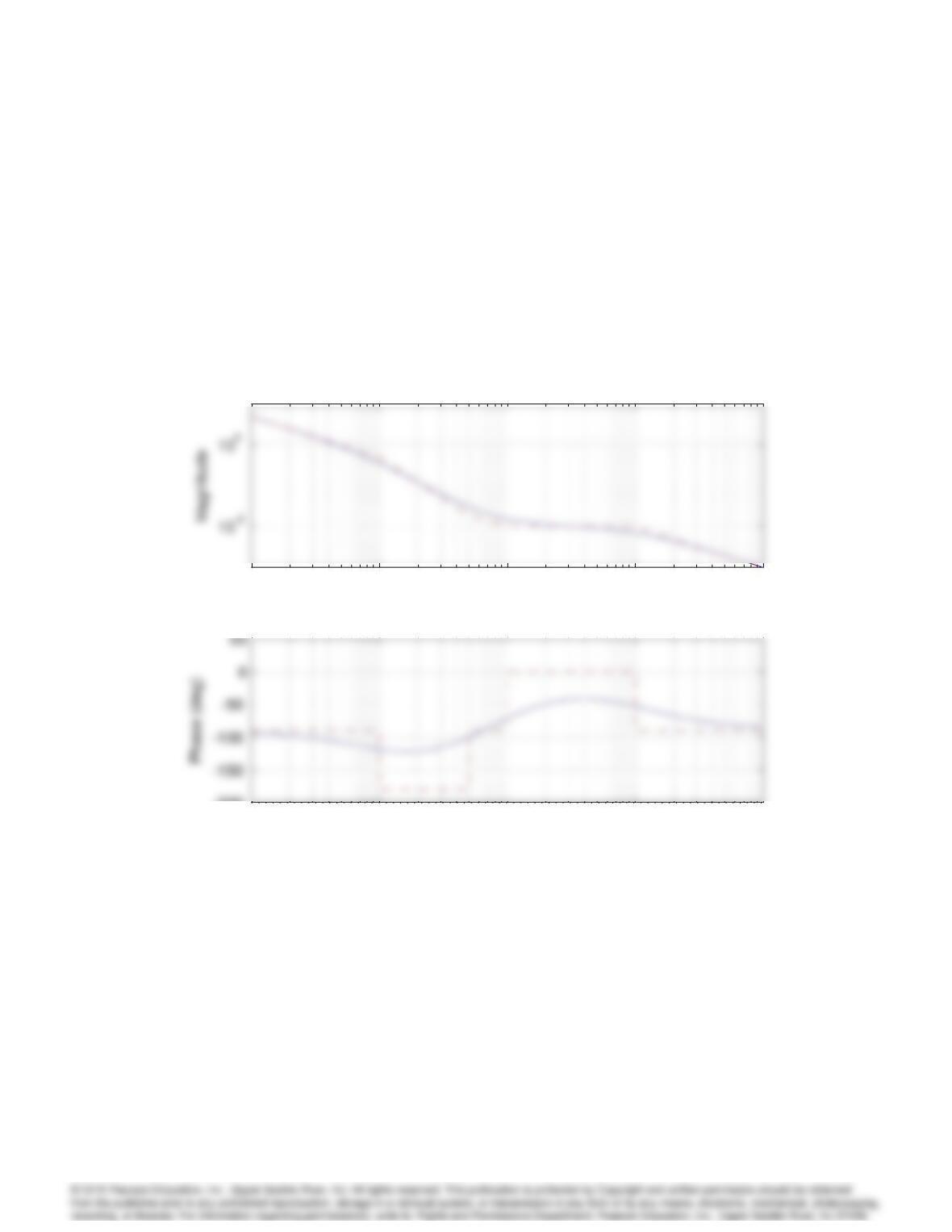
6011
10-1 100101102103
ω(rad/sec)
Bode plot for Prob 6.3(g)
10-1 100101102103
-200
ω (rad/sec)
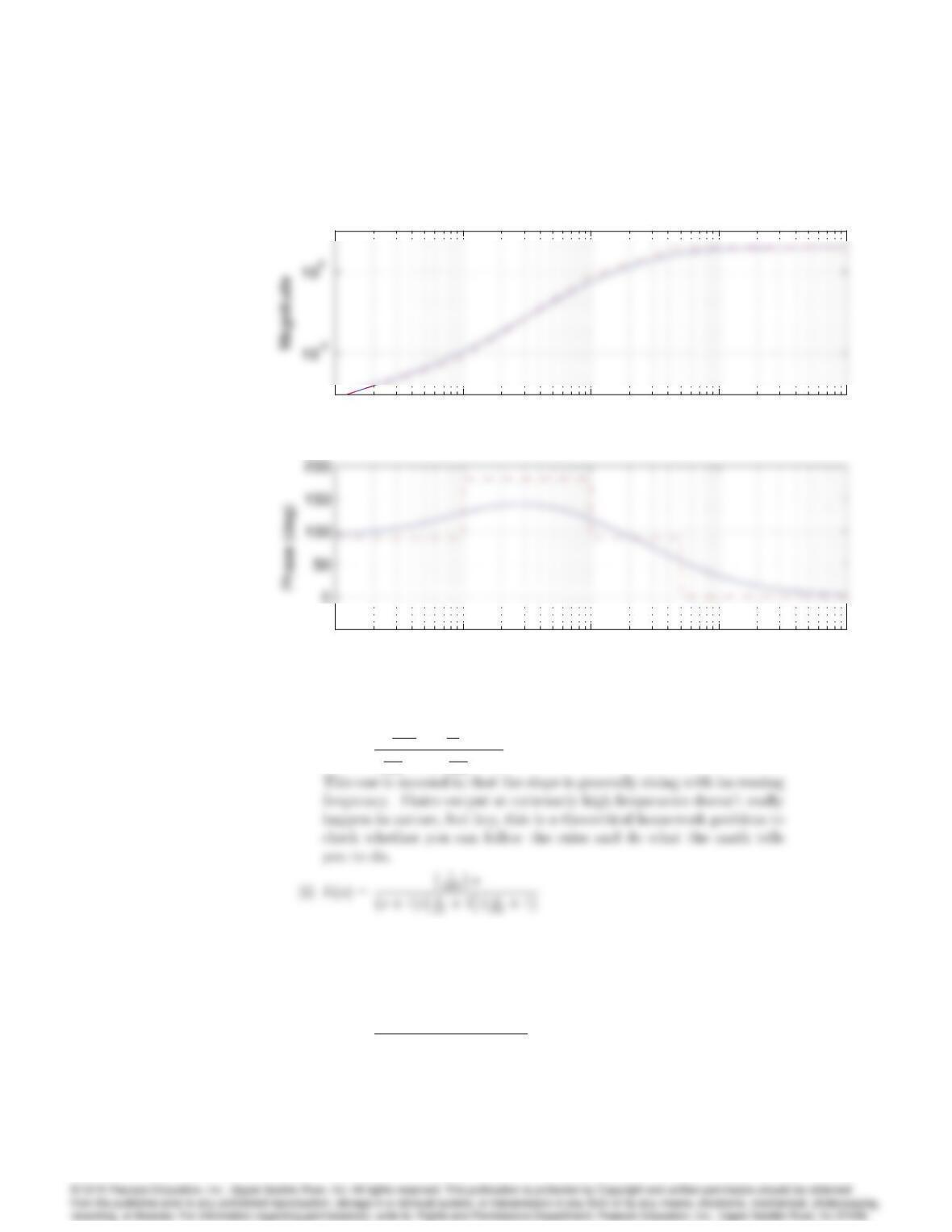
6012 CHAPTER 6. THE FREQUENCY-RESPONSE DESIGN METHOD
100101102103104
ω (rad/sec)
Bode plot for Prob 6.3(h)
100101102103104
-50
ω (rad/sec)
(h) L(s) = 4
5000 ss
10 + 1
s
100 + 1 s
500 + 1
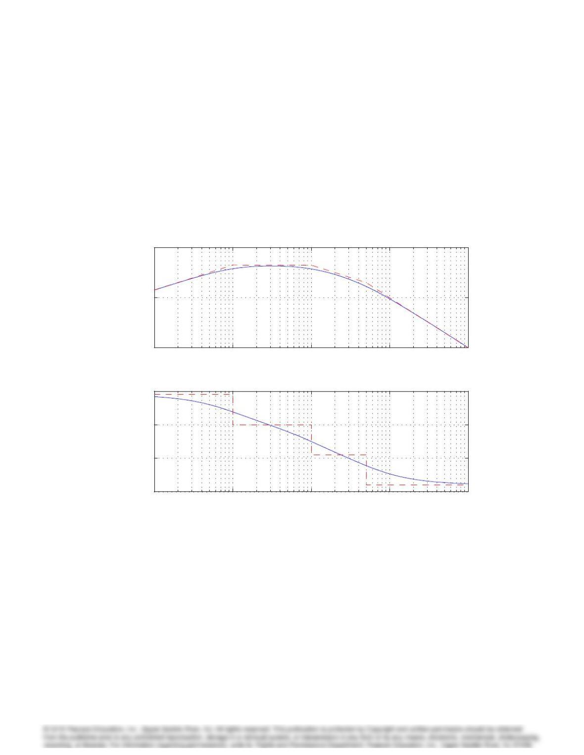
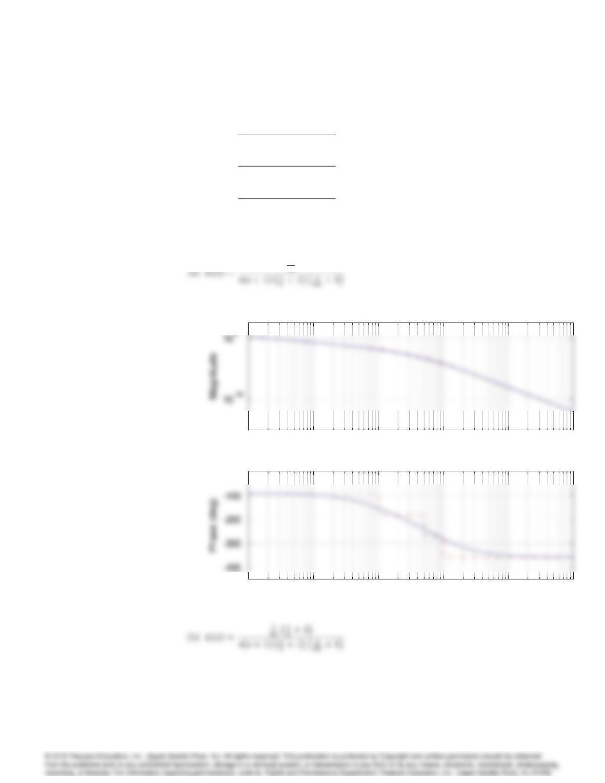
4. Real poles and zeros. Sketch the asymptotes of the Bode plot magnitude
and phase for each of the following open-loop transfer functions. After
completing the hand sketches verify your result using MATLAB. Turn in
your hand sketches and the MATLAB results on the same scales.
(a) L(s) = 1
s(s+ 1)(s+ 5)(s+ 10)
6013
10-1 100101102103
10-6
10-4
10-2
ω (rad/sec)
Magnitude
Bode plot for Prob 6.3(i)
10-1 100101102103
-200
-100
0
100
ω (rad/sec)
Phase (deg)
6014 CHAPTER 6. THE FREQUENCY-RESPONSE DESIGN METHOD
(b) L(s) = (s+ 2)
s(s+ 1)(s+ 5)(s+ 10)
(c) L(s) = (s+ 2)(s+ 6)
s(s+ 1)(s+ 5)(s+ 10)
(d) L(s) = (s+ 2)(s+ 4)
s(s+ 1)(s+ 5)(s+ 10)
Solution:
1
50
10-2 10-1 100101102103
ω (rad/sec)
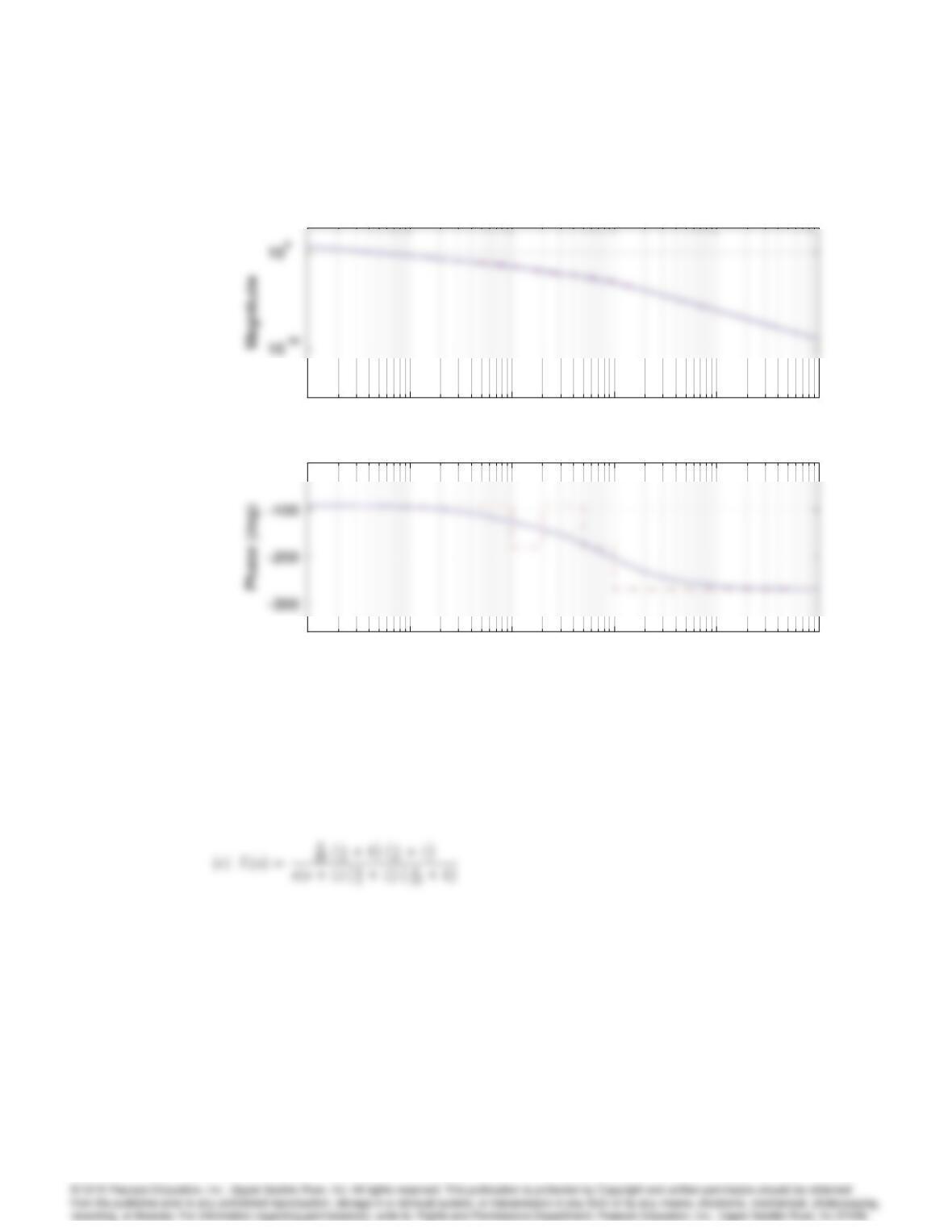
Bode plot for Prob. 6.4 (a)
10-2 10-1 100101102103
ω (rad/sec)
Bode plot for Prob. 6.4 (a)
10-2 10-1 100101102103
0
Frequency (rad/sec)
10-2 10-1 100101102103
ω (rad/sec)
Bode plot for Prob. 6.4 (a)
10-2 10-1 100101102103
ω (rad/sec)
Bode plot for Prob. 6.4 (a)
10-2 10-1 100101102103
0
Frequency (rad/sec)
6015
10-2 10-1 100101102103
ω (rad/sec)
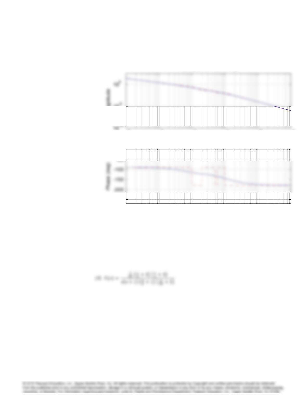
Bode plot for Prob. 6.4 (b)
10-2 10-1 100101102103
ω (rad/sec)
Bode plot for Prob. 6.4 (b)
10-2 10-1 100101102103
0
ω (rad/sec)
10-2 10-1 100101102103
ω (rad/sec)
Bode plot for Prob. 6.4 (b)
10-2 10-1 100101102103
ω (rad/sec)
Bode plot for Prob. 6.4 (b)
10-2 10-1 100101102103
0
ω (rad/sec)
6016 CHAPTER 6. THE FREQUENCY-RESPONSE DESIGN METHOD
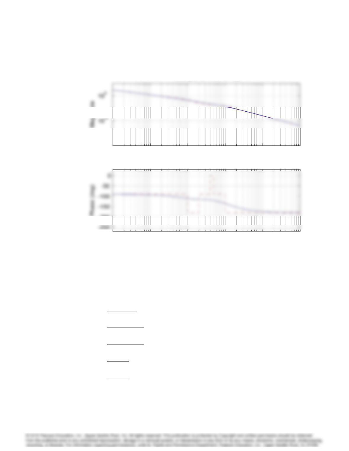
10-2 10-1 100101102103
10-5
ω (rad/sec)
Magnitude
Bode plot for Prob. 6.4 (c)
10-2 10-1 100101102103
10-5
ω (rad/sec)
Magnitude
Bode plot for Prob. 6.4 (c)
10-2 10-1 100101102103
-250
0
ω (rad/sec)
10-2 10-1 100101102103
10-5
ω (rad/sec)
Magnitude
Bode plot for Prob. 6.4 (c)
10-2 10-1 100101102103
10-5
ω (rad/sec)
Magnitude
Bode plot for Prob. 6.4 (c)
10-2 10-1 100101102103
-250
0
ω (rad/sec)
6017
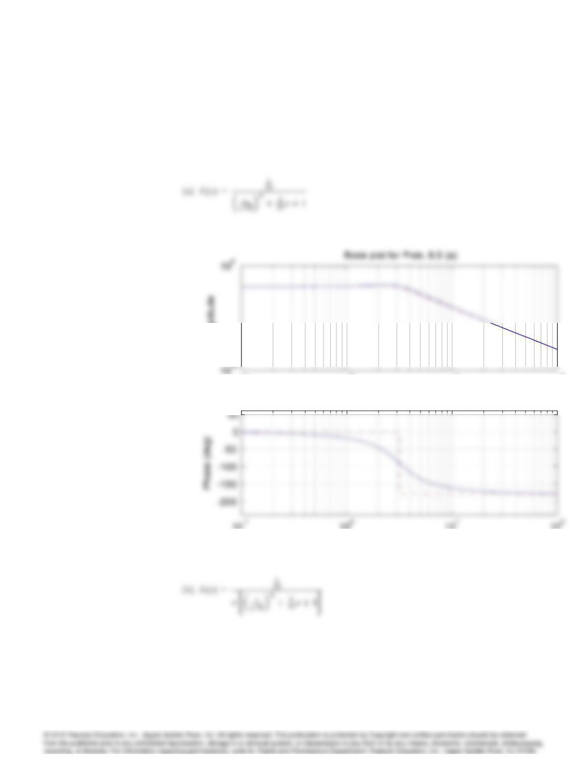
10-2 10-1 100101102103
10-10
ω (rad/sec)
Bode plot for Prob. 6.4 (d)
10-2 10-1 100101102103
10-10
ω (rad/sec)
Bode plot for Prob. 6.4 (d)
10-2 10-1 100101102103
-200
ω (rad/sec)
Phase (deg)
10-2 10-1 100101102103
10-10
ω (rad/sec)
Bode plot for Prob. 6.4 (d)
10-2 10-1 100101102103
10-10
ω (rad/sec)
Bode plot for Prob. 6.4 (d)
10-2 10-1 100101102103
-200
ω (rad/sec)
Phase (deg)
5. Complex poles and zeros Sketch the asymptotes of the Bode plot mag-
nitude and phase for each of the following open-loop transfer functions
and approximate the transition at the second order break point based
on the value of the damping ratio. After completing the hand sketches
verify your result using MATLAB. Turn in your hand sketches and the
MATLAB results on the same scales.
(a) L(s) = 1
s2+ 3s+ 10
(b) L(s) = 1
s(s2+ 3s+ 10)
(c) L(s) = (s2+ 2s+ 8)
s(s2+ 2s+ 10)
(d) L(s) = (s2+ 1)
s(s2+ 4)
(e) L(s) = (s2+ 4)
s(s2+ 1)
6018 CHAPTER 6. THE FREQUENCY-RESPONSE DESIGN METHOD
Solution:
10-1 100101102
ω (rad/sec)
Magnitude
10-1 100101102
ω (rad/sec)
Magnitude
10-1 100101102
ω (rad/sec)
10-1 100101102
ω (rad/sec)
Magnitude
10-1 100101102
ω (rad/sec)
Magnitude
10-1 100101102
ω (rad/sec)
6019
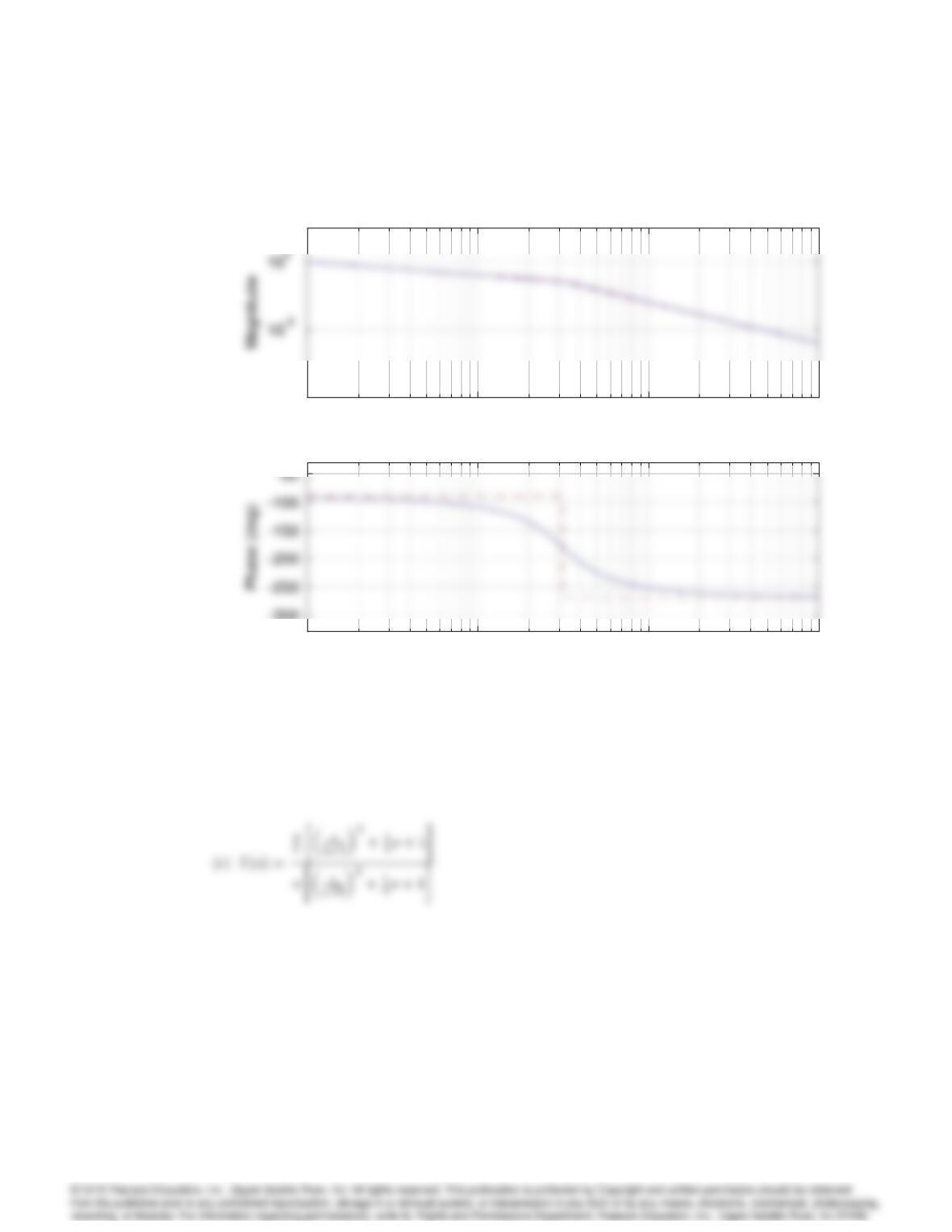
10-1 100101102
10-10
ω (rad/sec)
Bode plot for Prob. 6.5 (b)
10-1 100101102
10-10
ω (rad/sec)
Bode plot for Prob. 6.5 (b)
10-1 100101102
-300
ω (rad/sec)
10-1 100101102
10-10
ω (rad/sec)
Bode plot for Prob. 6.5 (b)
10-1 100101102
10-10
ω (rad/sec)
Bode plot for Prob. 6.5 (b)
10-1 100101102
-300
ω (rad/sec)