–16 –14 –12 –10 -8 -6 -4 -2 0 2
–0.8
–0.4
0.2
0.4
0.8
Real Axis
(b)
6061
10-4
102
Bode plot for Prob. 6.17(b)
10-4
102
Bode plot for Prob. 6.17(b)
10-1 100101102
-160
-120
ω (rad/sec)
Phase (deg)
10-4
102
Bode plot for Prob. 6.17(b)
10-4
102
Bode plot for Prob. 6.17(b)
10-1 100101102
-160
-120
ω (rad/sec)
Phase (deg)
(c)
6062 CHAPTER 6. THE FREQUENCY-RESPONSE DESIGN METHOD
–12 – 10 -8 -6 -4 -2 0 2
-6
8
Root Locus
Real Axis
6063
10-1 100101102
10-5
105
ω (rad/sec)
Magnitude
Bode plot for Fig. 6.17 (c)
10-1 100101102
10-5
105
ω (rad/sec)
Magnitude
Bode plot for Fig. 6.17 (c)
10-1 100101102
-100
150
ω (rad/sec)
10-1 100101102
10-5
105
ω (rad/sec)
Magnitude
Bode plot for Fig. 6.17 (c)
10-1 100101102
10-5
105
ω (rad/sec)
Magnitude
Bode plot for Fig. 6.17 (c)
10-1 100101102
-100
150
ω (rad/sec)
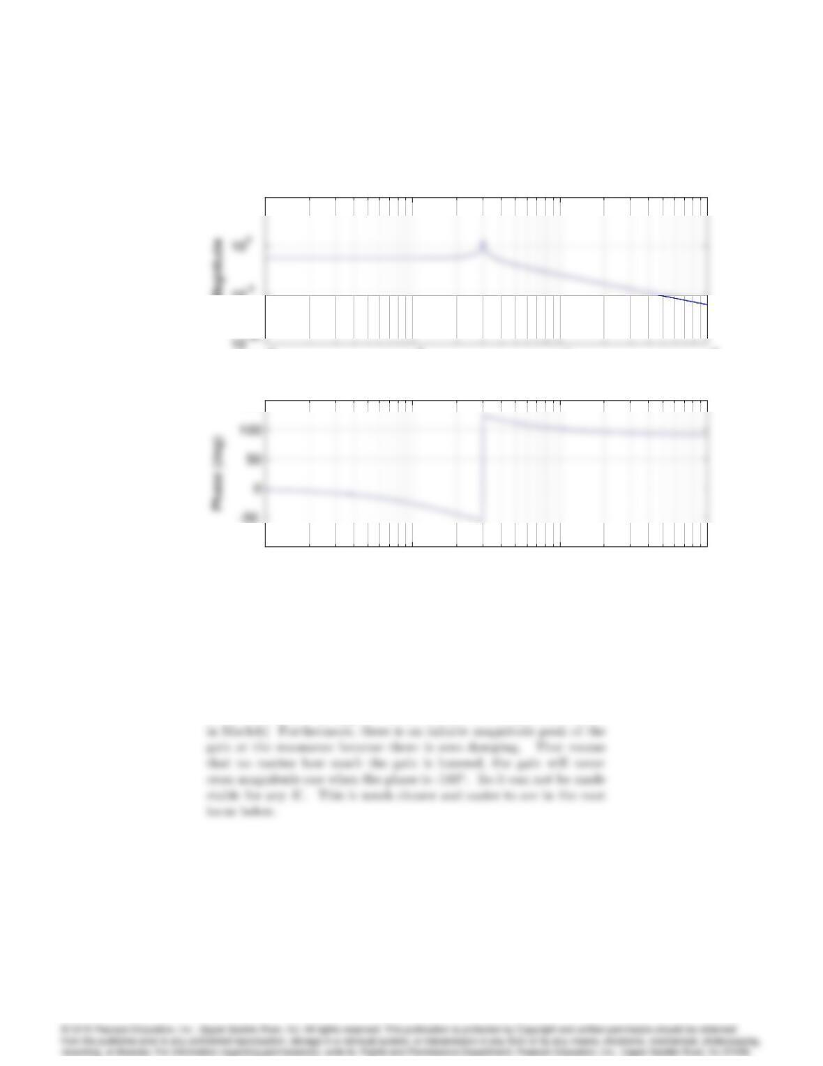
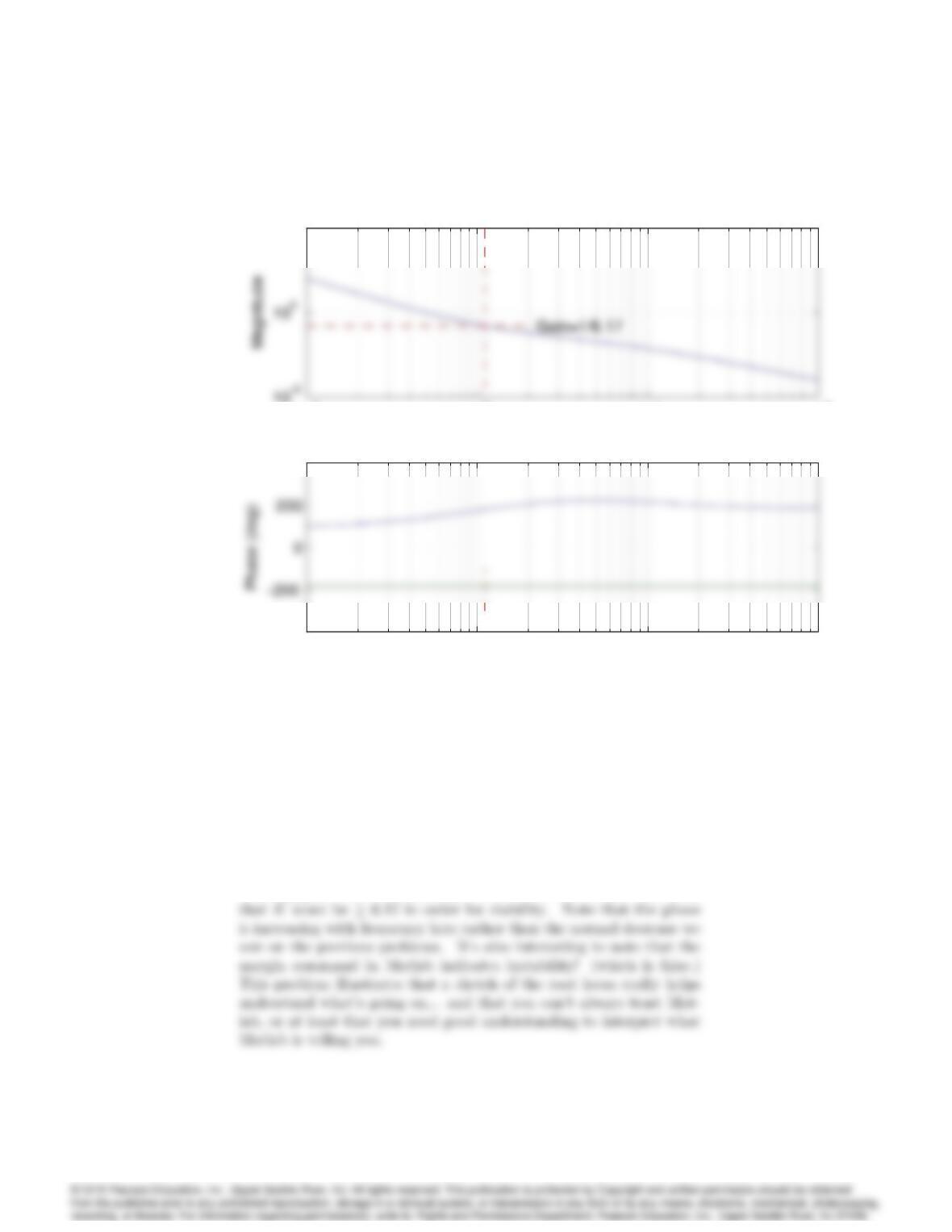
The bode is difficult to read, but the phase really dropped by 180o
at the resonance. (It appears to rise because of the quadrant action
6064 CHAPTER 6. THE FREQUENCY-RESPONSE DESIGN METHOD
–20 – 15 –10 -5 0 5 10
–15
15
Root Locus
Real Axis
(d)
6065
10-1 100101102
10-5
105
ω (rad/sec)
Bode plot for Prob. 6.17 (d)
10-1 100101102
10-5
105
ω (rad/sec)
Bode plot for Prob. 6.17 (d)
10-1 100101102
-400
400
ω (rad/sec)
10-1 100101102
10-5
105
ω (rad/sec)
Bode plot for Prob. 6.17 (d)
10-1 100101102
10-5
105
ω (rad/sec)
Bode plot for Prob. 6.17 (d)
10-1 100101102
-400
400
ω (rad/sec)
This is not the normal situation discussed in Section 6.2 where in-
creasing gain leads to instability. Here we see from the root locus
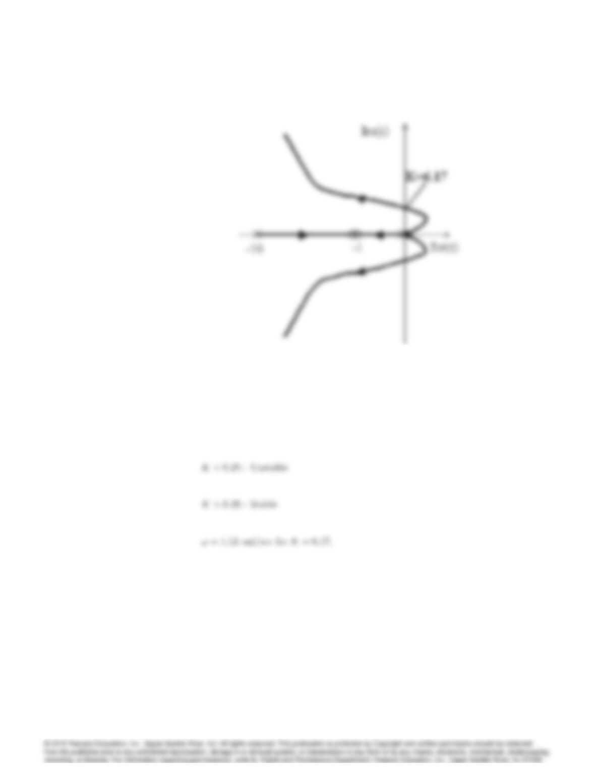
6066 CHAPTER 6. THE FREQUENCY-RESPONSE DESIGN METHOD
6067
Problems and Solutions for Section 6.3
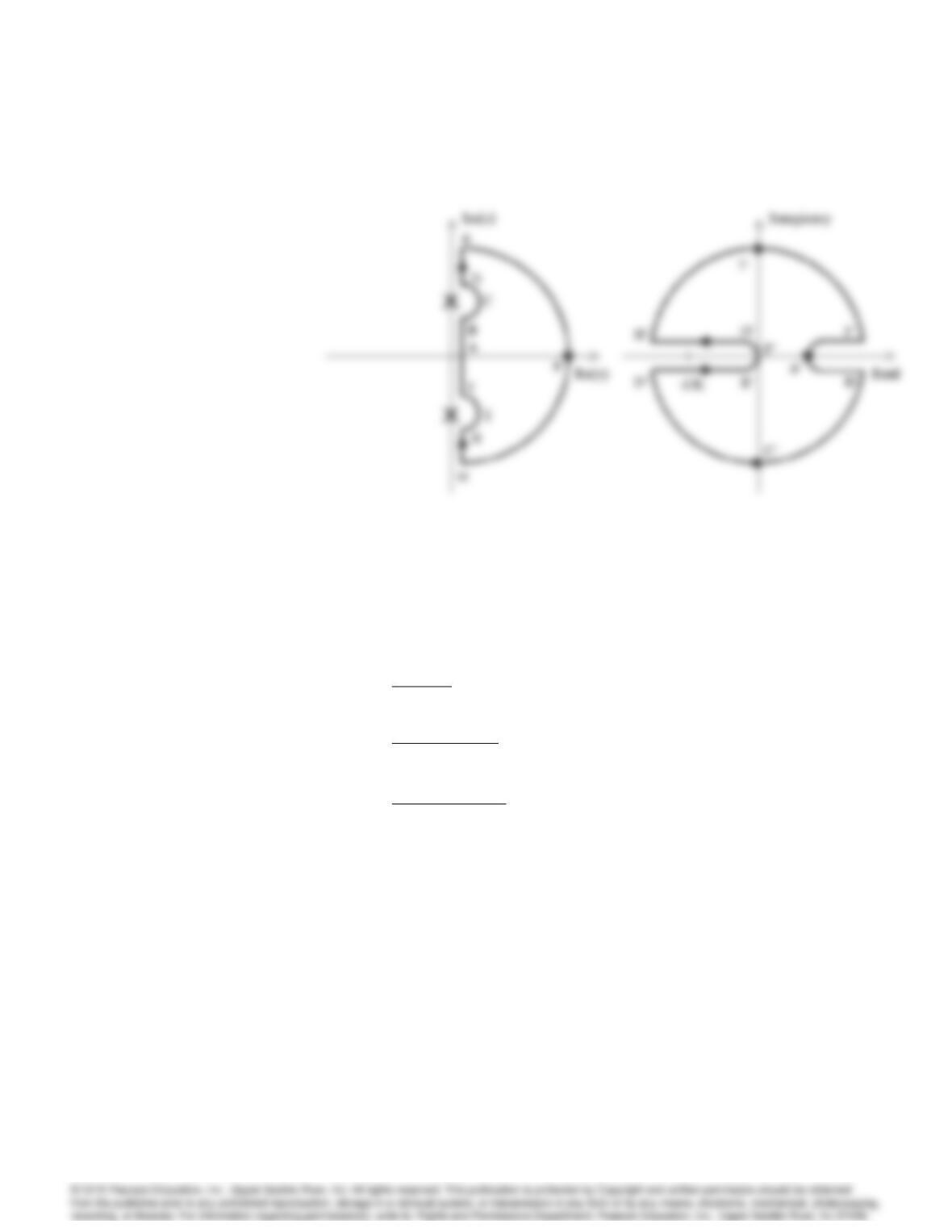
18. (a) Sketch the Nyquist plot for an open-loop system with transfer func-
tion 1=s2; that is, sketch 1
s2js=C1;
where C1is a contour enclosing the entire RHP, as shown in Fig. 6.17.
(Hint : Assume C1takes a small detour around the poles at s= 0, as
shown in Fig. 6.27.)
(b) Repeat part (a) for an open-loop system whose transfer function is
G(s) = 1=(s2+!2
0).
Solution :
(a)
G(s) = 1
s2
(b)
6068 CHAPTER 6. THE FREQUENCY-RESPONSE DESIGN METHOD
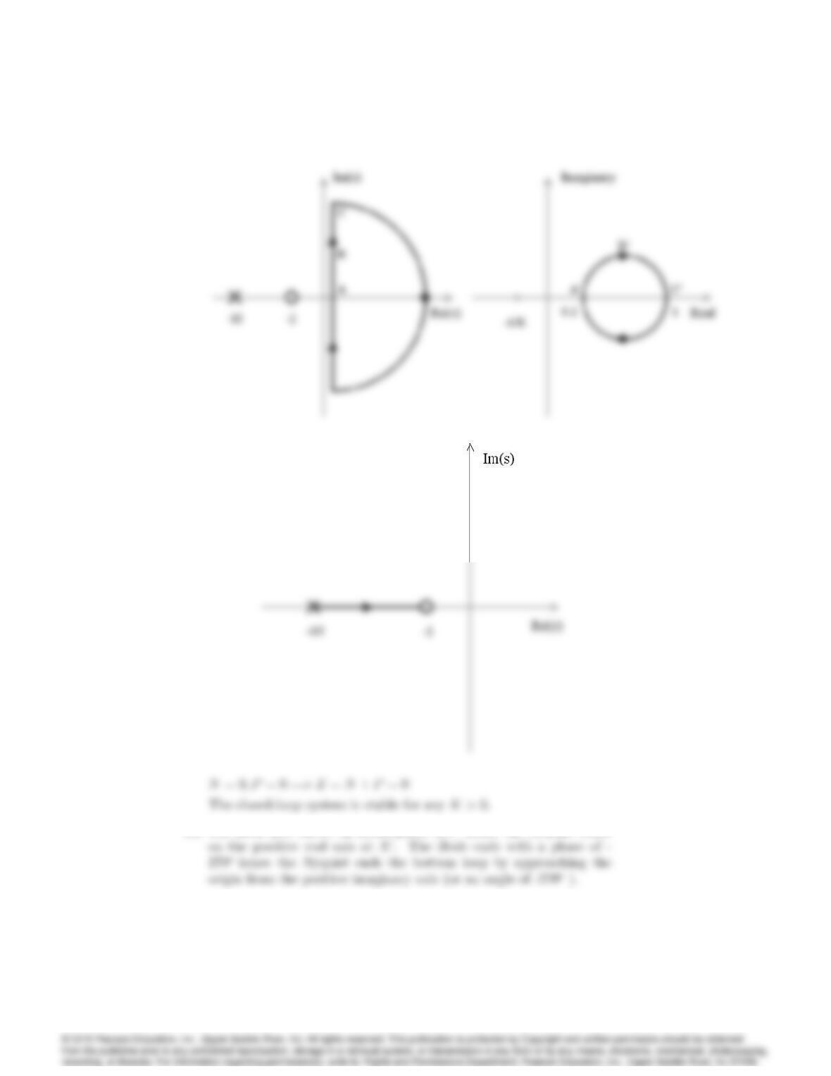
19. Sketch the Nyquist plot based on the Bode plots for each of the following
systems, then compare your result with that obtained using the MATLAB
command nyquist:
(a) KG(s) = K(s+ 2)
s+ 10
(b) KG(s) = K
(s+ 10)(s+ 2)2
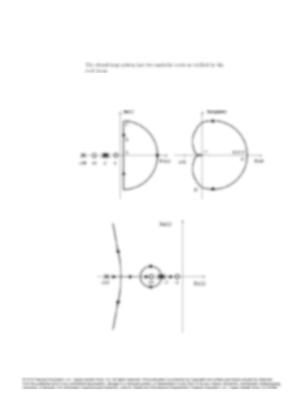
(c) KG(s) = K(s+ 10)(s+ 1)
(s+ 100)(s+ 2)3
(d) Using your plots, estimate the range of Kfor which each system is
stable, and qualitatively verify your result using a rough sketch of a
root-locus plot.
Solution :
(a)
6069
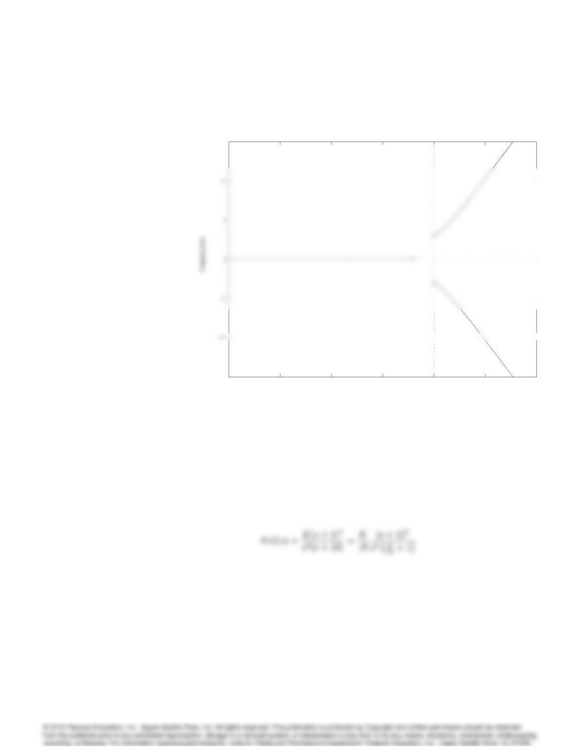
(b) The Bode plot shows an initial phase of 0ohence the Nyquist starts
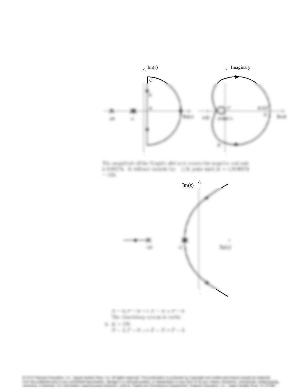
6070 CHAPTER 6. THE FREQUENCY-RESPONSE DESIGN METHOD
i. 0< K < 576
6071
(c) The Bode plot shows an initial phase of 0ohence the Nyquist starts
on the positive real axis at A’. The Bode ends with a phase of –
180ohence the Nyquist ends the bottom loop by approaching the
origin from the negative real axis (or an angle of -180o).
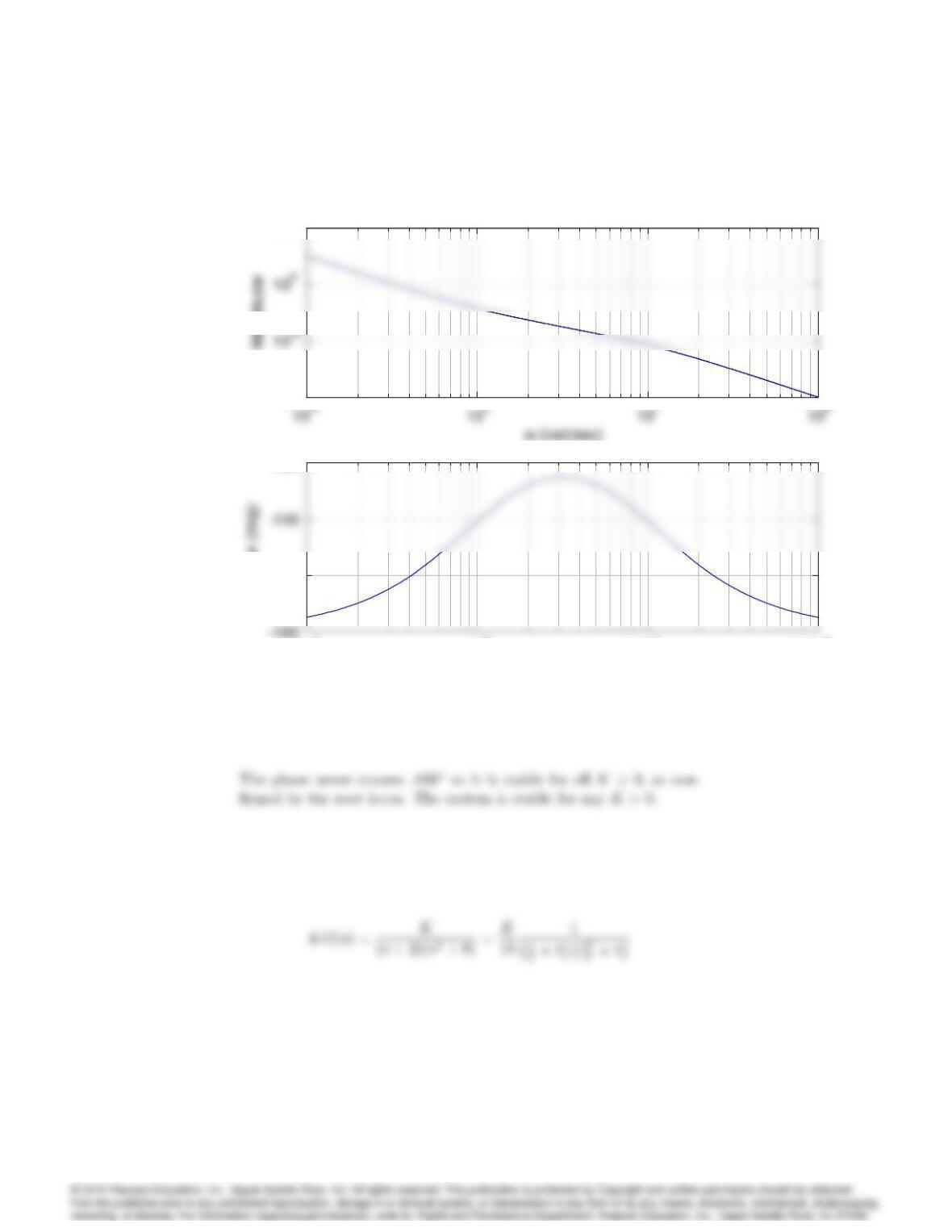
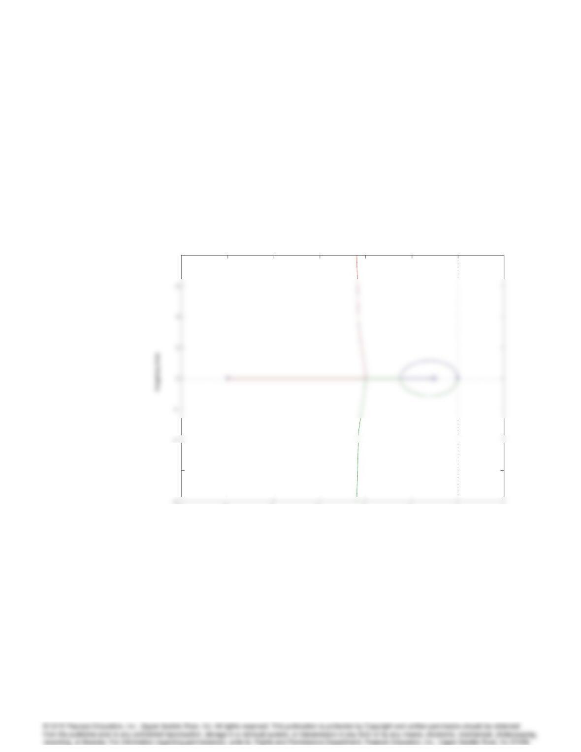
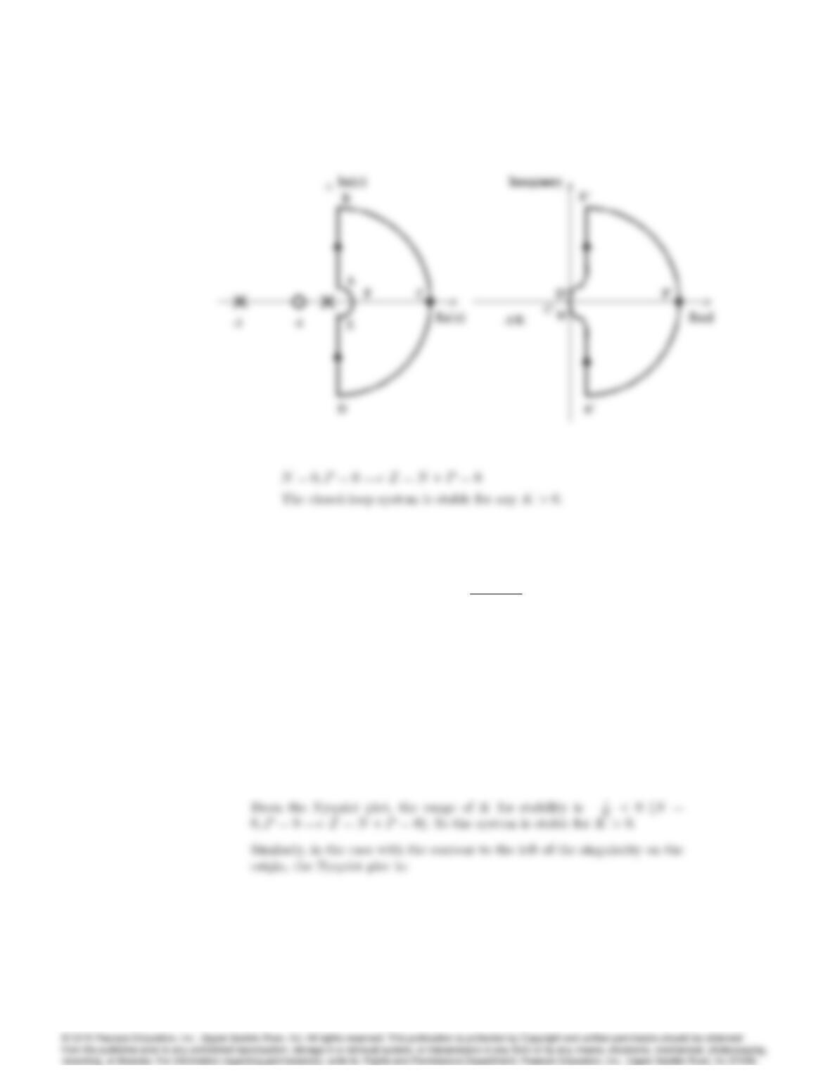
It will never encircle the -1/K point, hence it is always stable. The
root locus below con…rms that.
6072 CHAPTER 6. THE FREQUENCY-RESPONSE DESIGN METHOD
20. Draw a Nyquist plot for
KG(s) = K(s+ 1)
s(s+ 3) (1)
choosing the contour to be to the right of the singularity on the j!-axis.
and determine the range of Kfor which the system is stable using the
Nyquist Criterion. Then redo the Nyquist plot, this time choosing the
contour to be to the left of the singularity on the imaginary axis and again
check the range of Kfor which the system is stable using the Nyquist
Criterion. Are the answers the same? Should they be?
Solution :
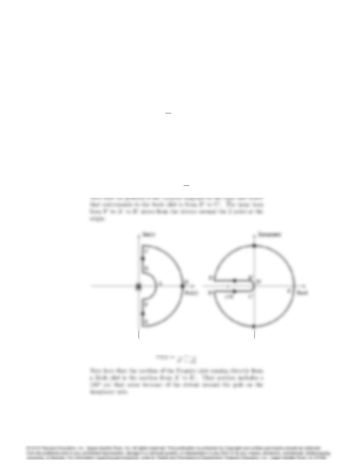
If you choose the contour to the right of the singularity on the origin, the
Nyquist plot looks like this :
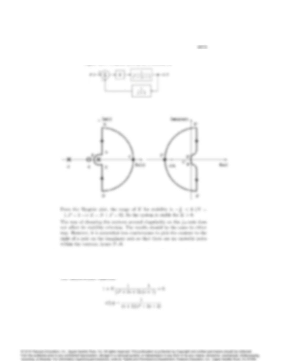
Figure 6.87: Control system for Problem 21
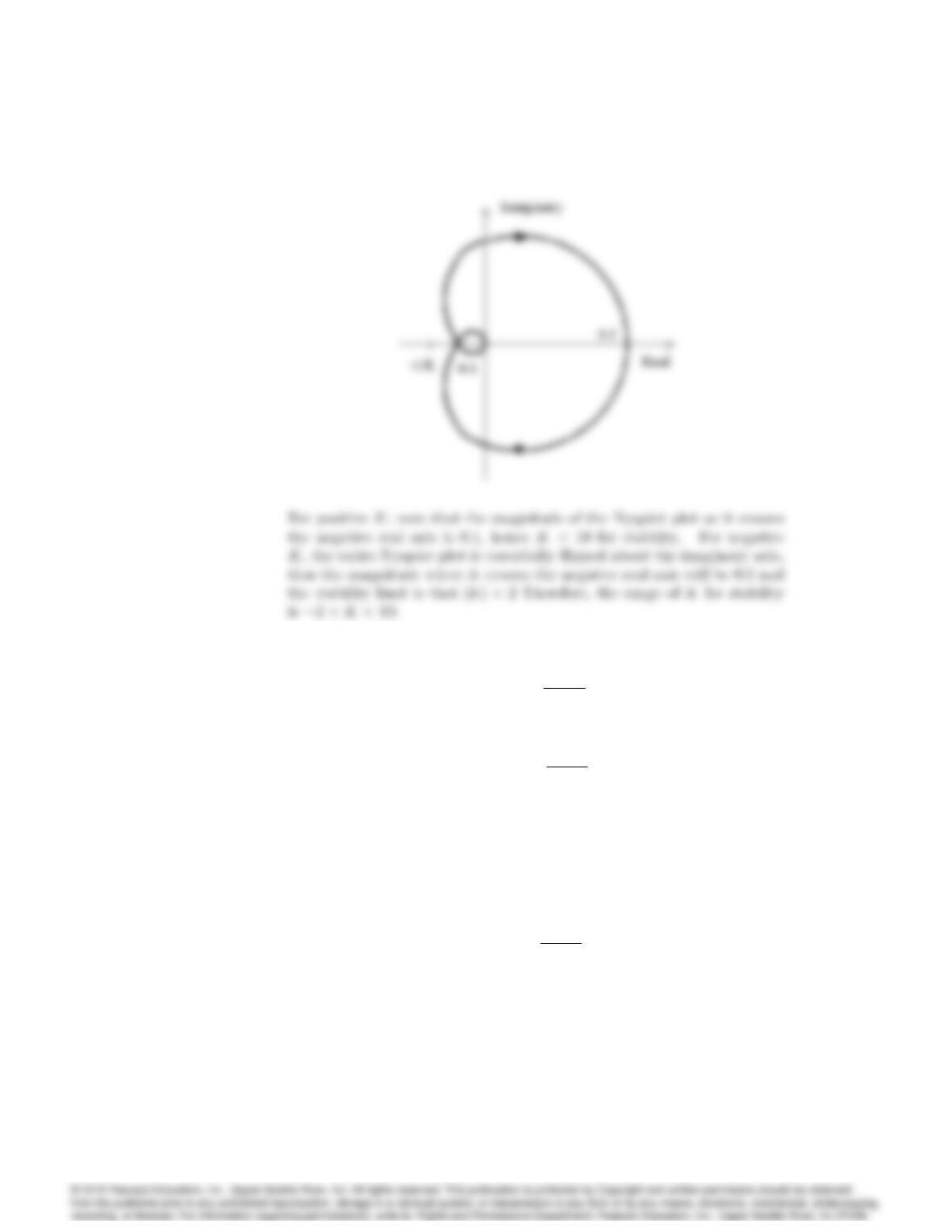
21. Draw the Nyquist plot for the system in Fig. 6.87. Using the Nyquist
stability criterion, determine the range of Kfor which the system is stable.
Consider both positive and negative values of K.
Solution :
6074 CHAPTER 6. THE FREQUENCY-RESPONSE DESIGN METHOD
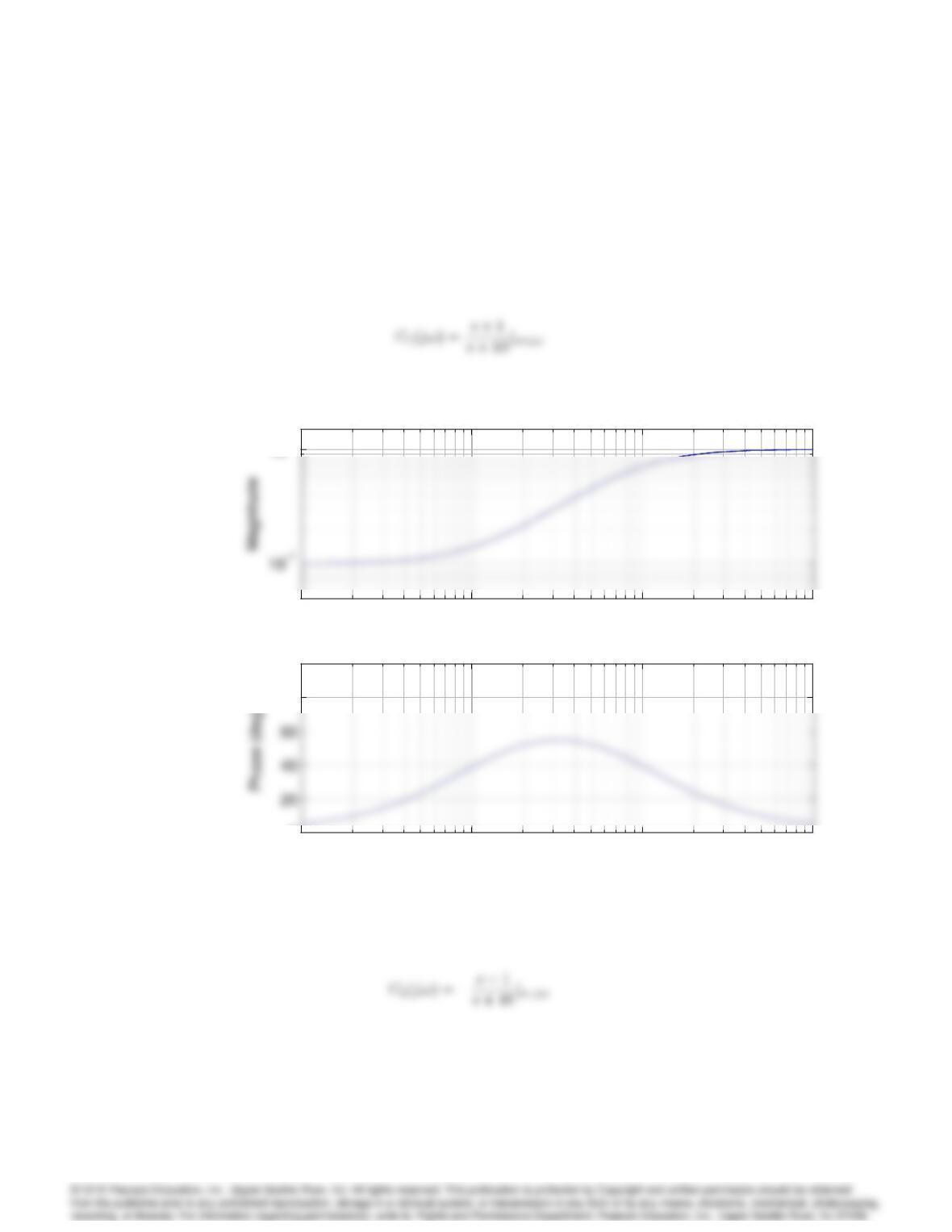
22. (a) For != 0:1to 100 rad/sec, sketch the phase of the minimum-phase
system
G(s) = s+ 1
s+ 10
s=j!
and the nonminimum-phase system
G(s) = s1
s+ 10
s=j!
;
noting that \(j! 1) decreases with !rather than increasing.
(b) Does a RHP zero affect the relationship between the 1 encirclements
on a polar plot and the number of unstable closed-loop roots in
Eq. (6.28)?
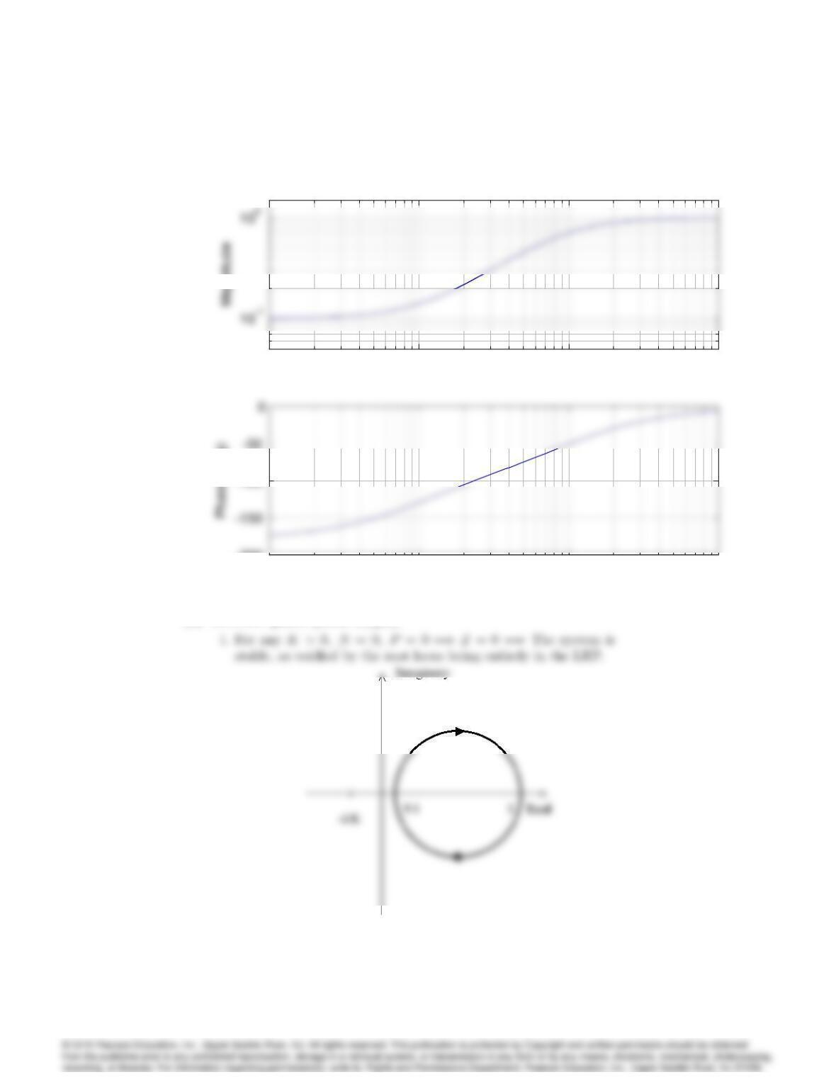
(c) Sketch the phase of the following unstable system for != 0:1to
100 rad/sec:
G(s) =
s+ 1
s10
s=j!
:
(d) Check the stability of the systems in (a) and (c) using the Nyquist
criterion on KG(s). Determine the range of Kfor which the closed-
loop system is stable, and check your results qualitatively using a
rough root-locus sketch.
6075
Solution :
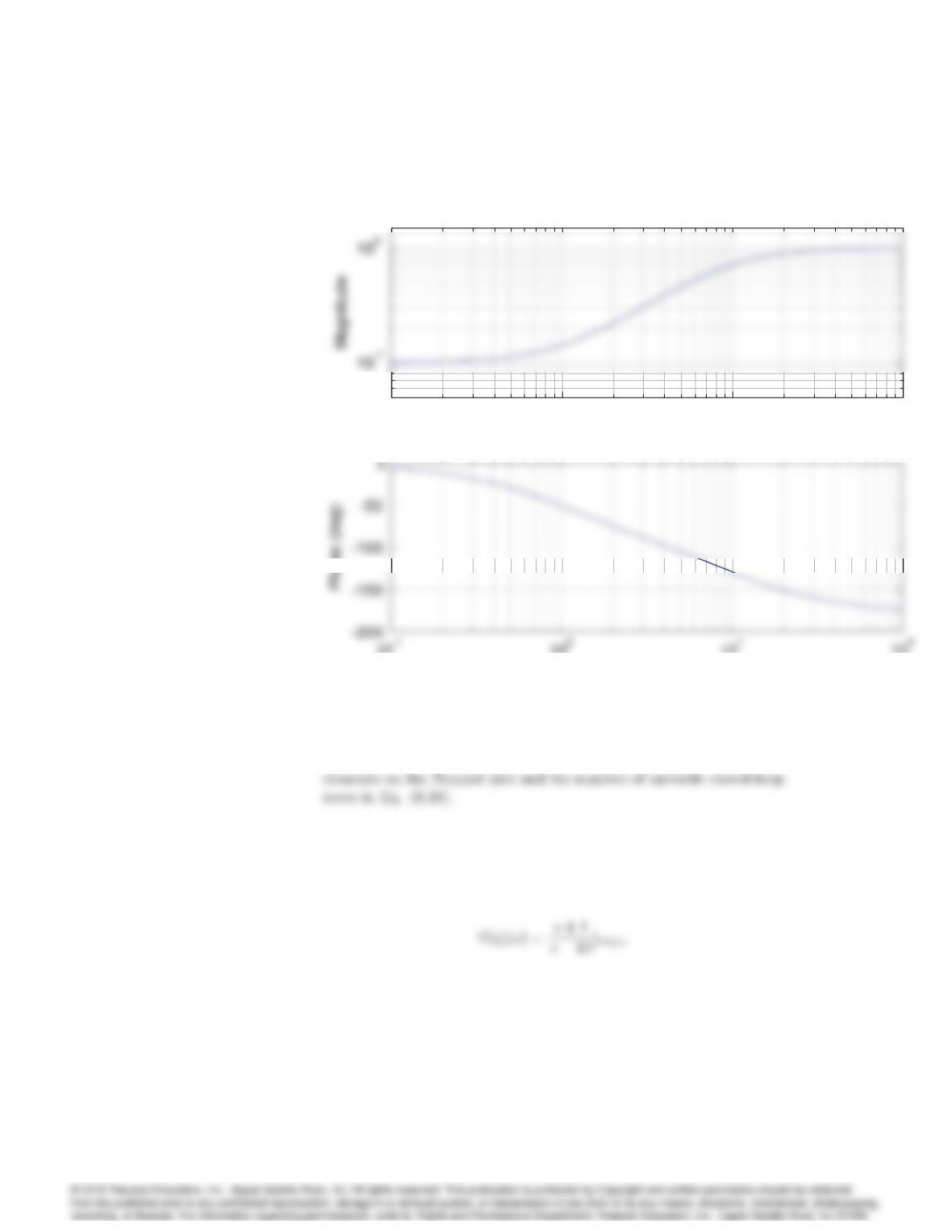
(a) Minimum phase system,
10-1 100101102
100
ω (rad/sec)
Bode plot for Prob. 6.22
10-1 100101102
100
ω (rad/sec)
Bode plot for Prob. 6.22
10-1 100101102
0
80
100
ω (rad/sec)
10-1 100101102
100
ω (rad/sec)
Bode plot for Prob. 6.22
10-1 100101102
100
ω (rad/sec)
Bode plot for Prob. 6.22
10-1 100101102
0
80
100
ω (rad/sec)
Non-minimum phase system,
6076 CHAPTER 6. THE FREQUENCY-RESPONSE DESIGN METHOD
10-1 100101102
ω (rad/sec)
Bode plot for Prob. 6.22
10-1 100101102
ω (rad/sec)
Bode plot for Prob. 6.22
10-1 100101102
ω (rad/sec)
10-1 100101102
ω (rad/sec)
Bode plot for Prob. 6.22
10-1 100101102
ω (rad/sec)
Bode plot for Prob. 6.22
10-1 100101102
ω (rad/sec)
(b) No, a RHP zero doesn’t affect the relationship between the 1encir-
(c) Unstable system:
6077
10-1 100101102
ω (rad/sec)
Bode plot for Prob. 6.22 (c)
10-1 100101102
ω (rad/sec)
Bode plot for Prob. 6.22 (c)
10-1 100101102
-200
-100
-50
ω (rad/sec)
10-1 100101102
ω (rad/sec)
Bode plot for Prob. 6.22 (c)
10-1 100101102
ω (rad/sec)
Bode plot for Prob. 6.22 (c)
10-1 100101102
-200
-100
-50
ω (rad/sec)
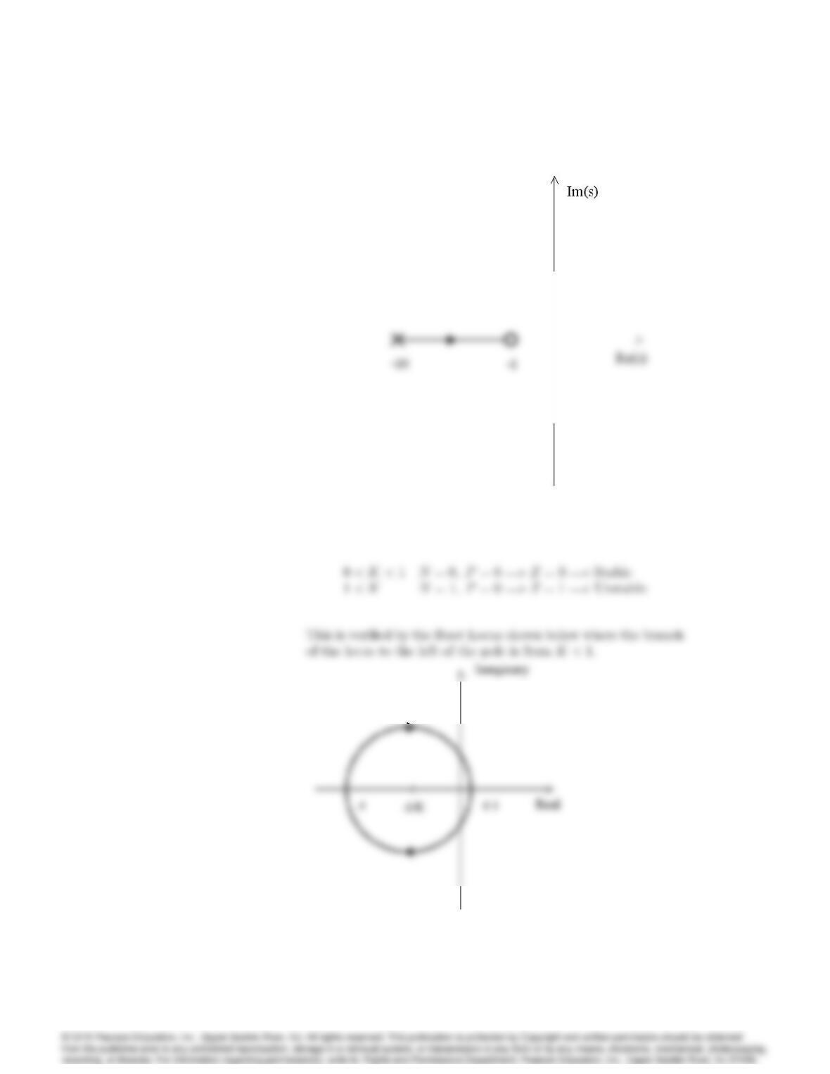
(d) Minimum phase system G1(j!):
6078 CHAPTER 6. THE FREQUENCY-RESPONSE DESIGN METHOD
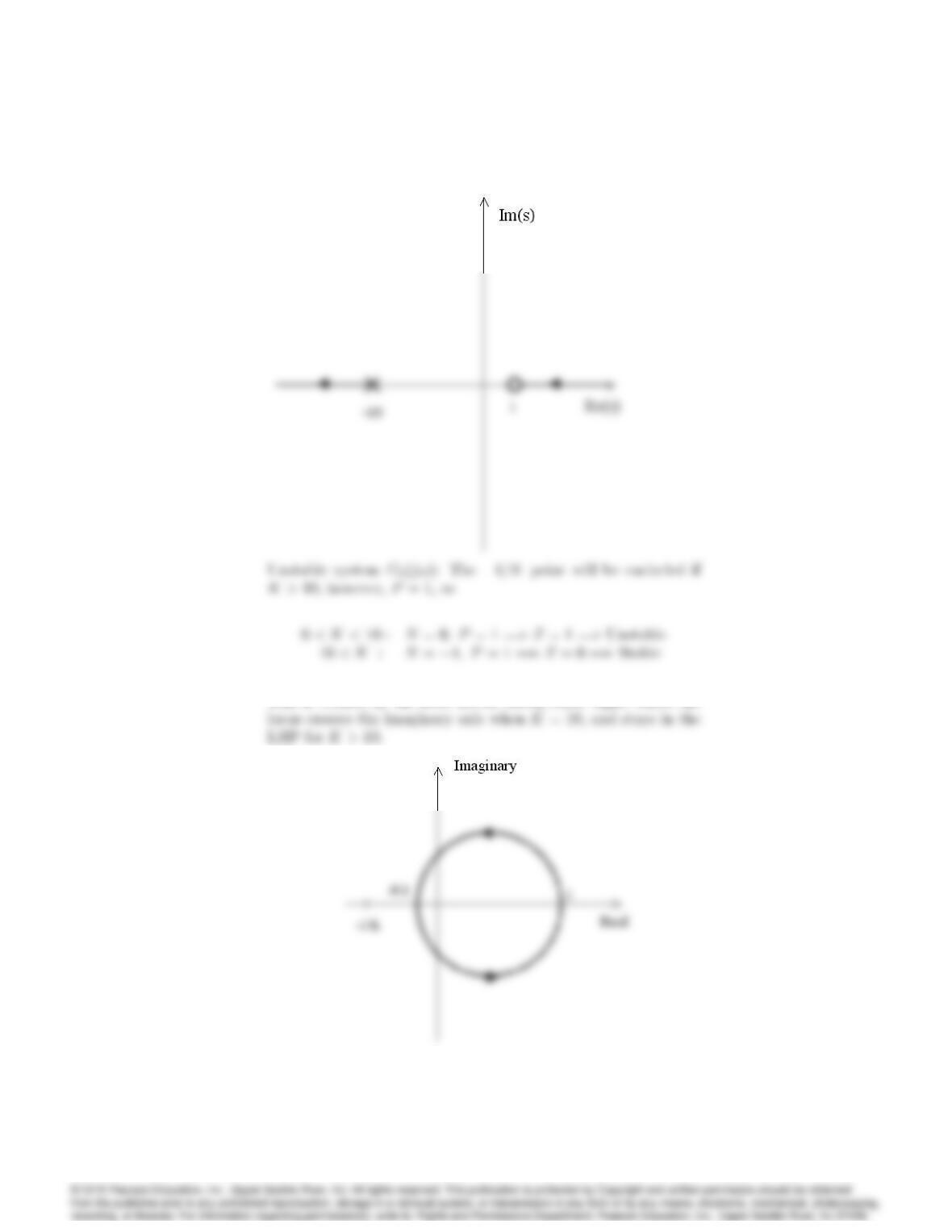
Non-minimum phase system G2(j!): the 1=K point will not
be encircled if K < 1:
6079
This is veri…ed by the Root Locus shown below right, where the