6120 CHAPTER 6. THE FREQUENCY-RESPONSE DESIGN METHOD
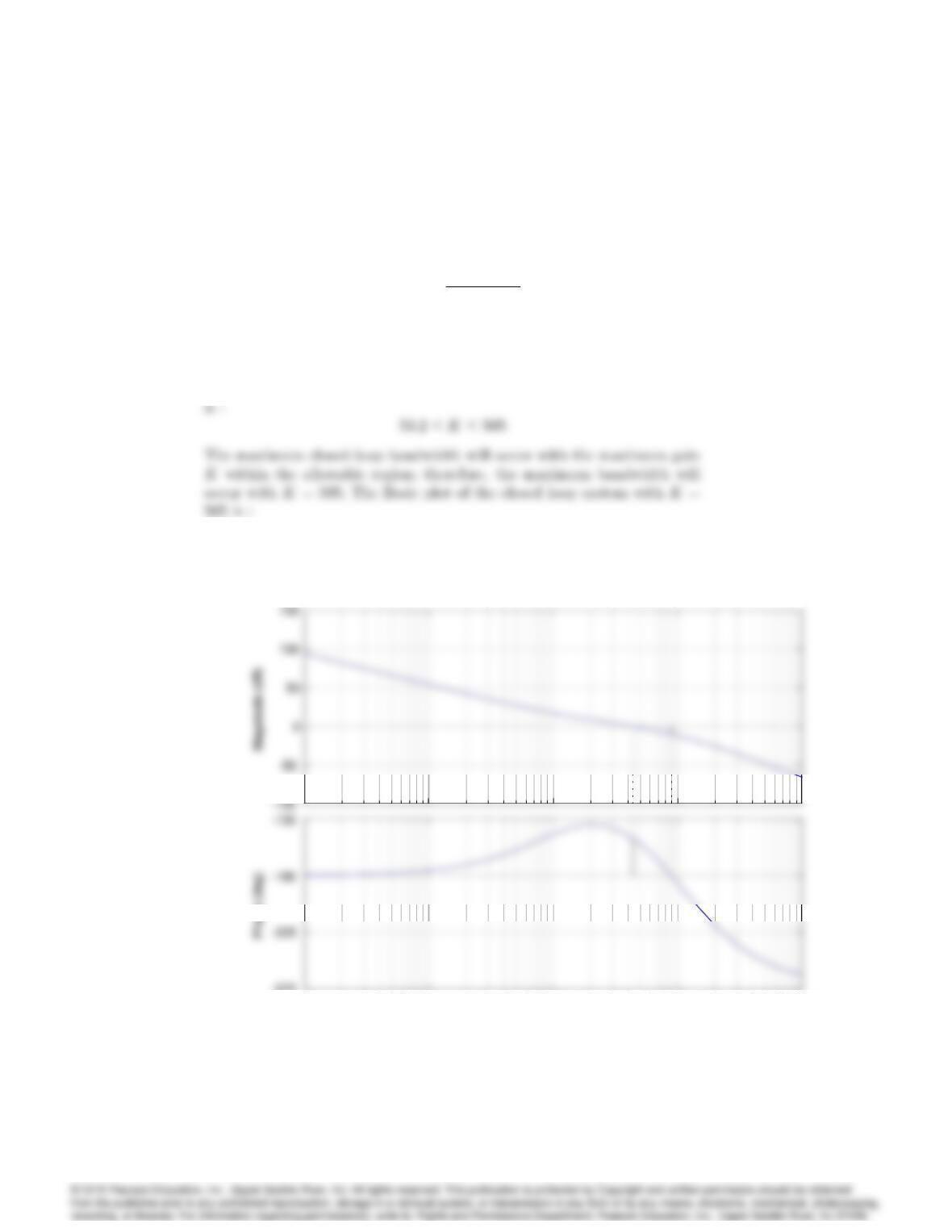
Note : Actual PM is as follows :
6121
Problem and Solution for Section 6.6
43. For the open-loop system
KG(s) = K(s+ 1)
s2(s+ 10)2:
Determine the value for Kthat will yield PM 30and the maximum
possible closed-loop bandwidth. Use MATLAB to find the bandwidth.
Solution :
From the result of Problem 6.40., the value of Kthat will yield P M 30
10
-2
10
-1
10
0
10
1
10
2
–270
Bode Diagram
Gm = 10 dB (at 8.94 rad/sec) , Pm = 30 deg (at 4.36 rad/sec)
Frequency (rad/sec)
10
-2
10
-1
10
0
10
1
10
2
–270
6122 CHAPTER 6. THE FREQUENCY-RESPONSE DESIGN METHOD
Problems and Solutions for Section 6.7
44. For the lead compensator
Dc(s) = TDs+ 1
TDs+ 1;
where < 1.
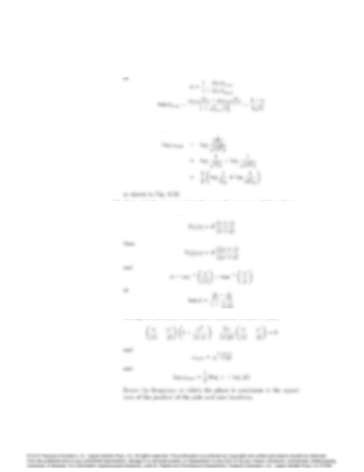
(a) Show that the phase of the lead compensator is given by
= tan1(TD!)tan1(TD!):
(b) Show that the frequency where the phase is maximum is given by
!max =1
TDp;
and that the maximum phase corresponds to
sin max =1
1 + :
(c) Rewrite your expression for !max to show that the maximum-phase
frequency occurs at the geometric mean of the two corner frequencies
on a logarithmic scale:
log !max =1
2log 1
TD
+ log 1
TD:
(d) To derive the same results in terms of the pole-zero locations, rewrite
Dc(s)as
Dc(s) = s+z
s+p;
and then show that the phase is given by
= tan1!
jzjtan1!
jpj;
such that
!max =pjzjjpj:
Hence the frequency at which the phase is maximum is the square
root of the product of the pole and zero locations.
6123
Solution :
(a) The frequency response is obtained by letting s=j!,
(b) Using the trigonometric relationship,
then
and since,
then
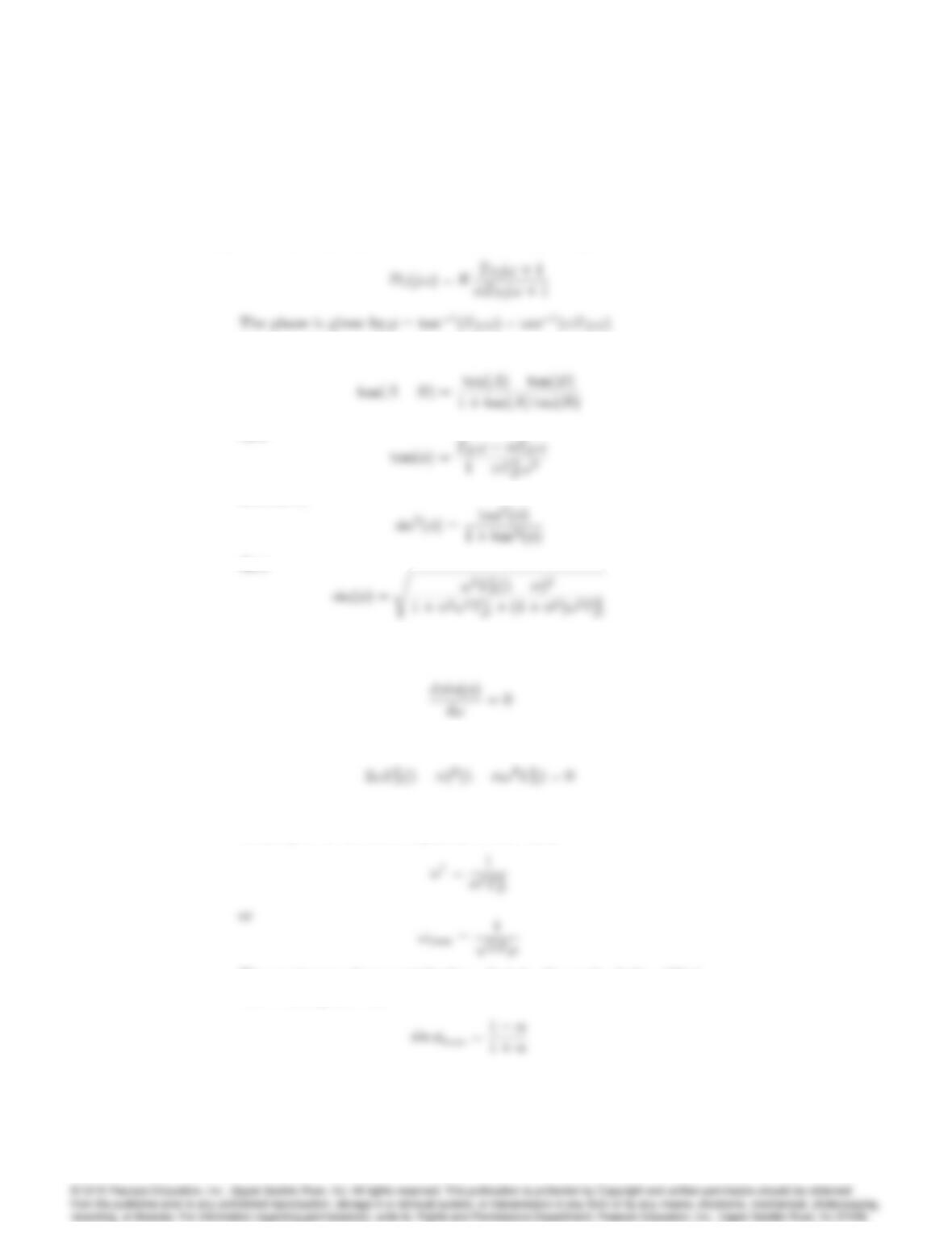
To determine the frequency at which the phase is a maximum, let us
set the derivative with respect to !equal to zero,
which leads to
The value != 0 gives the maximum of the function and setting the
second part of the above equation to zero then,
The maximum phase contribution, that is, the peak of the \D(s)
curve corresponds to,
6124 CHAPTER 6. THE FREQUENCY-RESPONSE DESIGN METHOD
(c) The maximum frequency occurs midway between the two break fre-
quencies on a logarithmic scale,
(d) Alternatively, we may state these results in terms of the pole-zero
locations. Rewrite Dc(s)as,
Setting the derivative of the above equation to zero we find,
45. For the third-order servo system
G(s) = 50;000
s(s+ 10)(s+ 50):
Design a lead compensator so that PM 50and !BW 20 rad/sec using
Bode plot sketches, then verify and refine your design using Matlab.
Solution :
The Bode plot of the given system is :
–100
10
-1
10
0
10
1
10
2
10
3
–225
Bode Diagram
Frequency (rad/sec)
–100
10
-1
10
0
10
1
10
2
10
3
–225
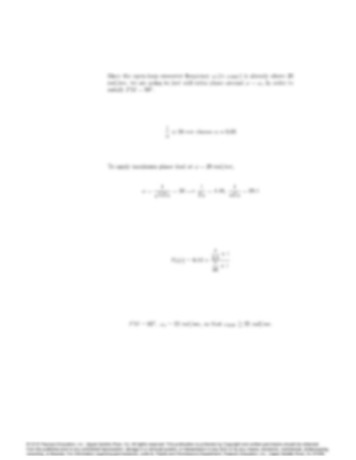
Start with a lead compensator design with :
6126 CHAPTER 6. THE FREQUENCY-RESPONSE DESIGN METHOD
Let’s add phase lead 60. From Fig. 6.53,
Therefore by applying the lead compensator with some gain adjustments
:
we get the compensated system with :
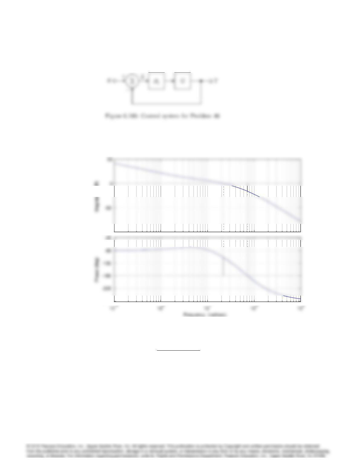
The Bode plot with designed compensator is :
6127
–100
–270
Bode Diagram
Gm = 15.9 dB (at 72.6 rad/sec) , Pm = 65.3 deg (at 22 rad/sec)
–100
–270
46. For the system shown in Fig. 6.100, suppose that
G(s) = 5
s(s+ 1)(s=5 + 1):
Design a lead compensation D(s)with unity DC gain so that PM 40
using Bode plot sketches, then verify and refine your design using Matlab.
What is the approximate bandwidth of the system?
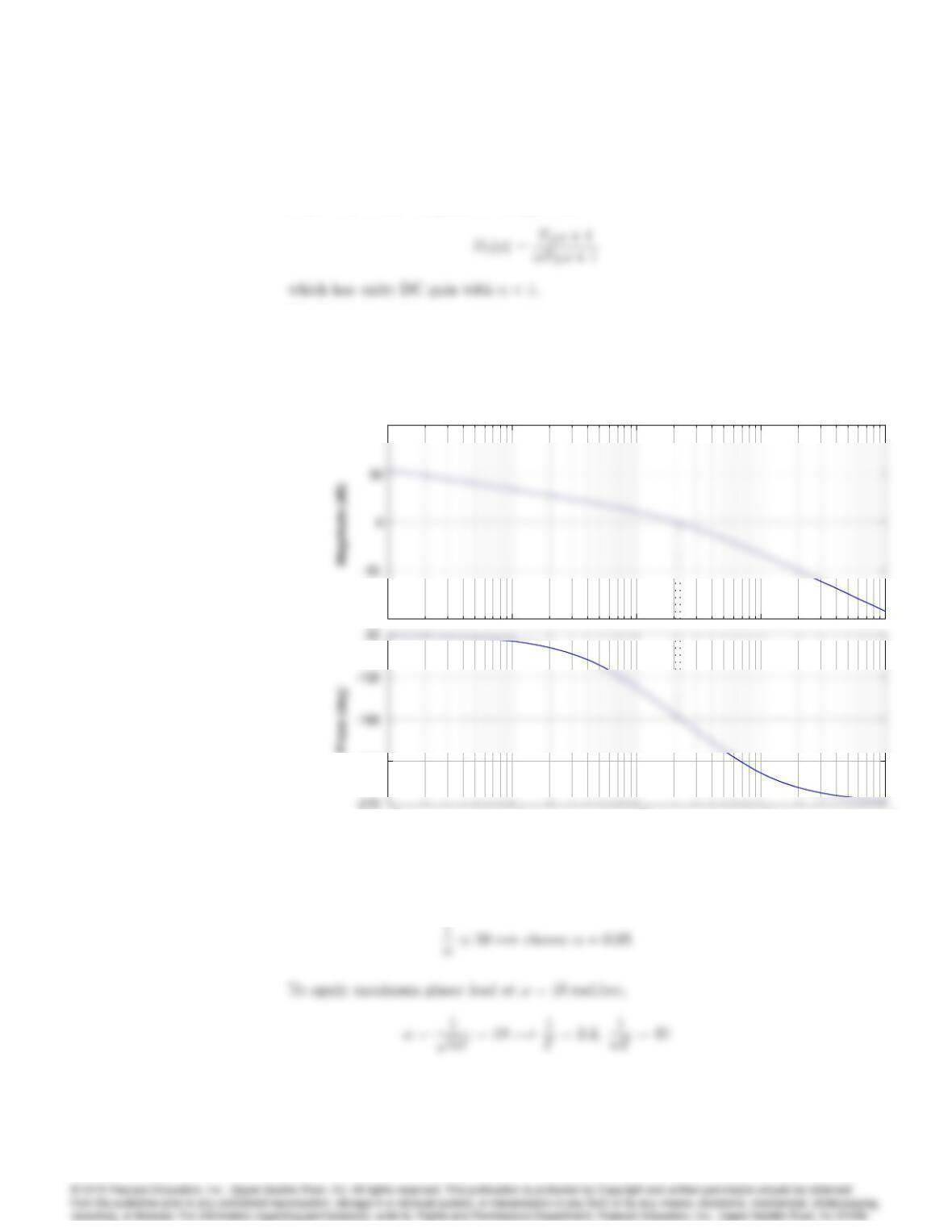
Solution :
6128 CHAPTER 6. THE FREQUENCY-RESPONSE DESIGN METHOD
Start with a lead compensator design with :
The Bode plot of the given system is :
–100
100
10
-2
10
-1
10
0
10
1
10
2
–225
Phase (deg)
Bode Diagram
Gm = 1.58 dB (at 2.24 rad/sec) , Pm = 3.94 deg (at 2.04 rad/sec)
Frequency (rad/sec)
–100
100
10
-2
10
-1
10
0
10
1
10
2
–225
Phase (deg)
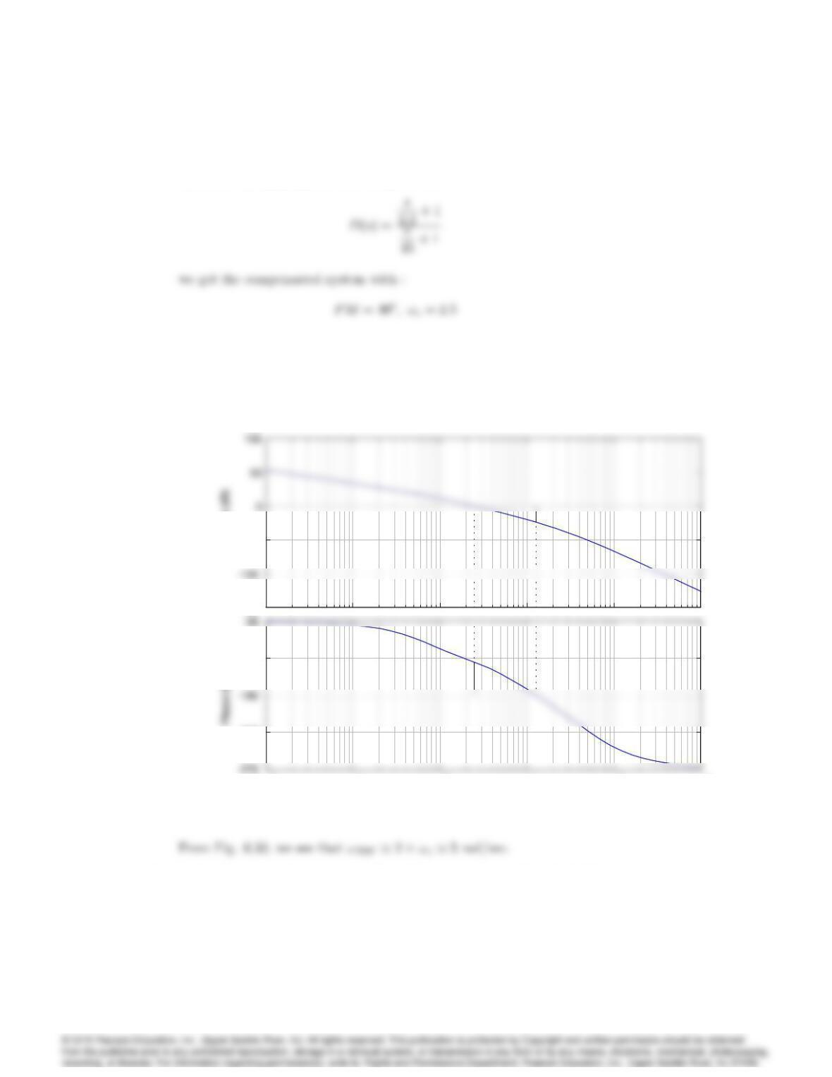
Since P M = 3:9, let’s add phase lead 60. From Fig. 6.53,
6129
Therefore by applying the lead compensator :
The Bode plot with designed compensator is :
–150
–50
Magnitude (dB)
10
-2
10
-1
10
0
10
1
10
2
10
3
–225
–135
Bode Diagram
Gm = 24.1 dB (at 12.8 rad/sec) , Pm = 40.2 deg (at 2.49 rad/sec)
Frequency (rad/sec)
–150
–50
Magnitude (dB)
10
-2
10
-1
10
0
10
1
10
2
10
3
–225
–135
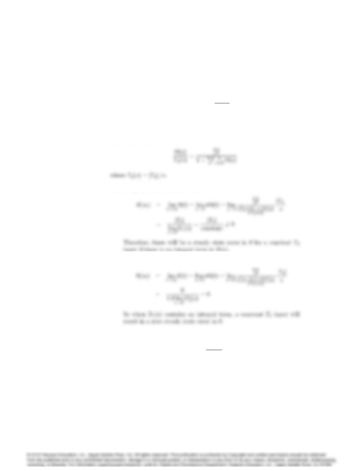
47. Derive the transfer function from Tdto for the system in Fig. 6.67. Then
apply the Final Value Theorem (assuming Td= constant) to determine
whether (1)is nonzero for the following two cases:
6130 CHAPTER 6. THE FREQUENCY-RESPONSE DESIGN METHOD
(a) When Dc(s)has no integral term: lims!0Dc(s) = constant;
(b) When Dc(s)has an integral term:
Dc(s) = D0
c(s)
s;
where lims!0D0
c(s) = constant.
Solution :
The transfer function from Tdto :
(a) Using the final value theorem :
input if there is no integral term in D(s).
(b)
48. The inverted pendulum has a transfer function given by Eq. (2.31), which
is similar to
G(s) = 1
s21:
(a) Design a lead compensator to achieve a PM of 30using Bode plot
sketches, then verify and refine your design using Matlab.
(b) Sketch a root locus and correlate it with the Bode plot of the system.
(c) Could you obtain the frequency response of this system experimen-
tally?
6131
Solution :
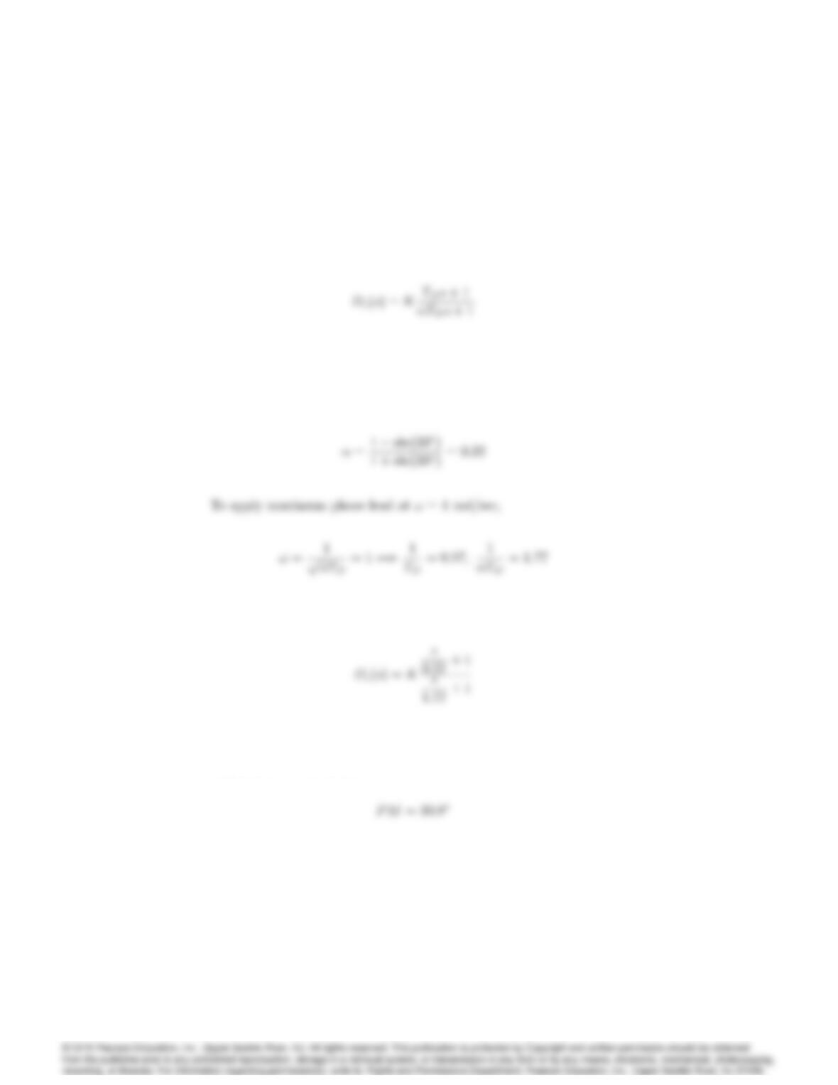
(a) Design the lead compensator :
such that the compensated system has P M ‘30&!c‘1rad/sec.
(Actually, the bandwidth or speed of response was not specified, so
any crossover frequency would satisfy the problem statement.)
Therefore by applying the lead compensator :
By adjusting the gain Kso that the crossover frequency is around 1
rad/sec, K= 1:13 results in :
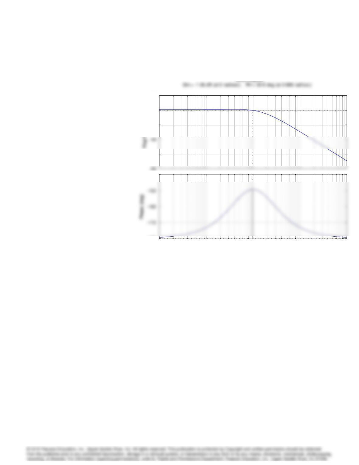
The Bode plot of compensated system is :
6132 CHAPTER 6. THE FREQUENCY-RESPONSE DESIGN METHOD
–60
–20
0
20
10
-2
10
-1
10
0
10
1
10
2
–180
–140
Bode Diagram
Frequency (rad/sec)
–60
–20
0
20
10
-2
10
-1
10
0
10
1
10
2
–180
–140
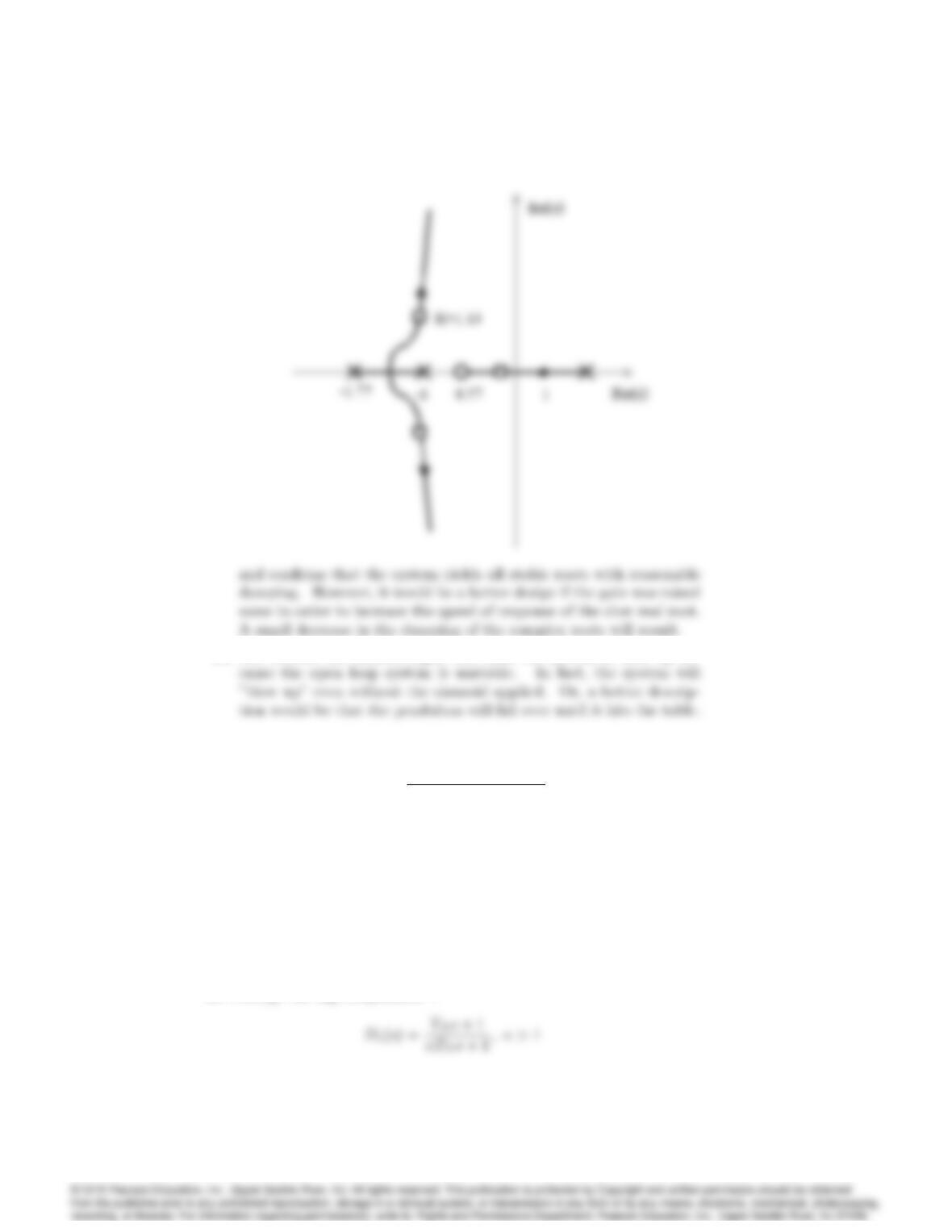
(b) Root Locus of the compensated system is :
6133
(c) No, because the sinusoid input will cause the system to blow up be-
49. The open-loop transfer function of a unity feedback system is
G(s) = K
s(s=5 + 1)(s=50 + 1):
(a) Design a lag compensator for G(s)using Bode plot sketches so that
the closed-loop system satisfies the following specifications:
i. The steady-state error to a unit ramp reference input is less than
0.01.
ii. PM = 40
(b) Verify and refine your design using Matlab.
Solution :
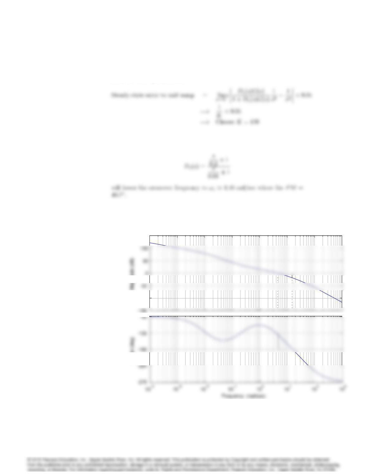
Let’s design the lag compensator :
6134 CHAPTER 6. THE FREQUENCY-RESPONSE DESIGN METHOD
From the first specification,
Uncompensated, the crossover frequency with K= 150 is too high for a
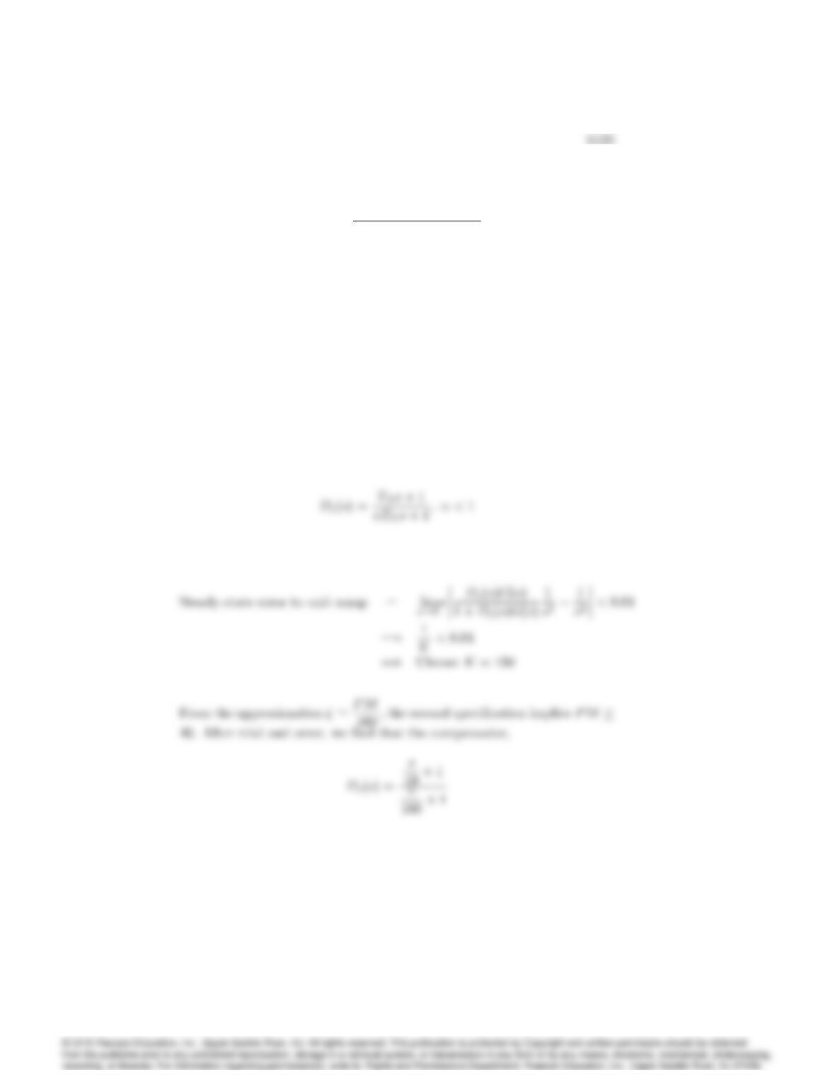
good P M . With some trial and error, we find that the lag compensator,
–100
150
Phase (deg)
Bode Diagram
Gm = 18.9 dB (at 15.5 rad/sec) , Pm = 40.7 deg (at 4.46 rad/sec)
–100
150
Phase (deg)
50. The open-loop transfer function of a unity feedback system is
G(s) = K
s(s=5 + 1)(s=200 + 1):
(a) Design a lead compensator for G(s)using Bode plot sketches so that
the closed-loop system satisfies the following specifications:
i. The steady-state error to a unit ramp reference input is less than
0.01.
ii. For the dominant closed-loop poles the damping ratio 0:4.
(b) Verify and refine your design using Matlab including a direct com-
putation of the damping of the dominant closed-loop poles.
Solution :
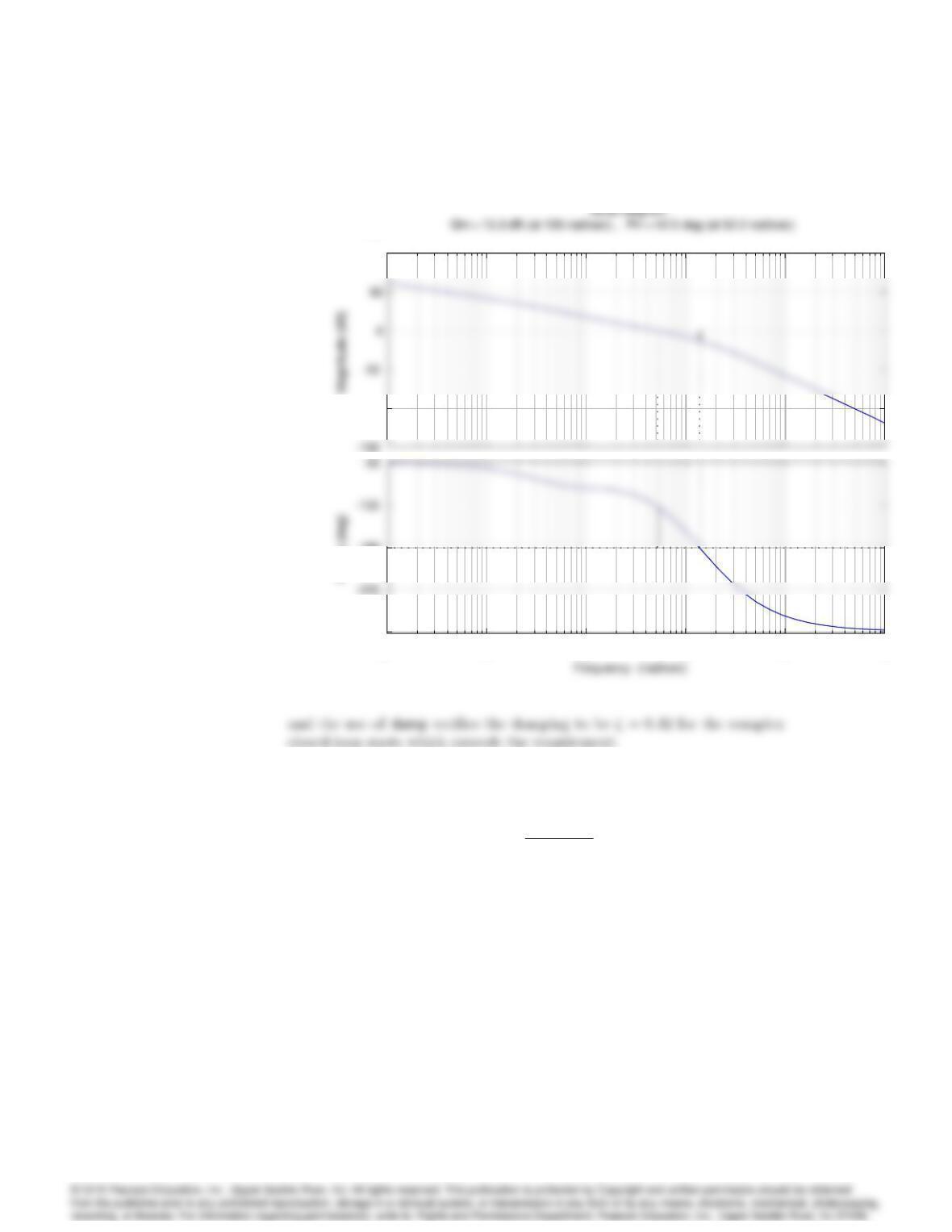
Let’s design the lead compensator :
From the first specification,
results in a P M = 42:5and a crossover frequency !c‘51:2rad/sec as
shown by the margin output:
6136 CHAPTER 6. THE FREQUENCY-RESPONSE DESIGN METHOD
–100
100
10
-1
10
0
10
1
10
2
10
3
10
4
–270
–180
–100
100
10
-1
10
0
10
1
10
2
10
3
10
4
–270
–180
51. A DC motor with negligible armature inductance is to be used in a position
control system. Its open-loop transfer function is given by
G(s) = 50
s(s=5 + 1):
(a) Design a compensator for the motor using Bode plot sketches so that
the closed-loop system satisfies the following specifications:
i. The steady-state error to a unit ramp input is less than 1/200.
ii. The unit step response has an overshoot of less than 20%.
iii. The bandwidth of the compensated system is no less than that
of the uncompensated system.
(b) Verify and/or refine your design using Matlab including a direct
computation of the step response overshoot.
6137
Solution :
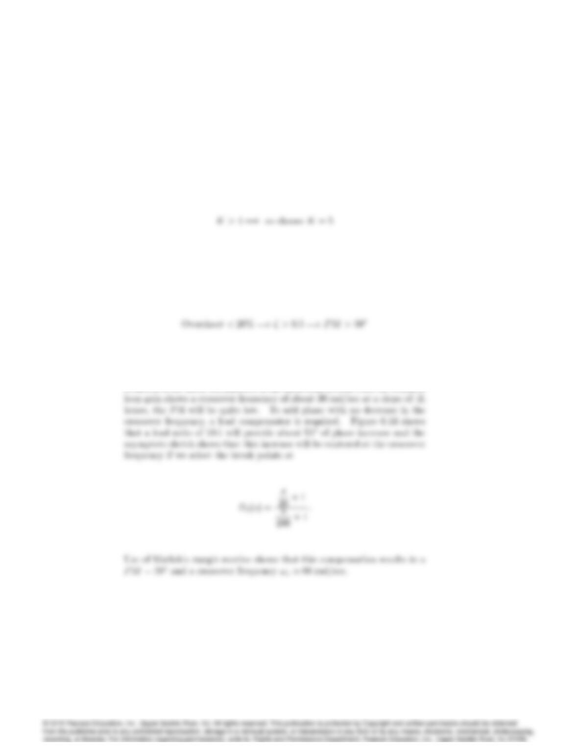
The first specification implies that a loop gain greater than 200 is required.
Since the open loop gain of the plant is 50, a gain from the compensator,
K; is required where
From Figure 3.24, we see that the second specification implies that :
A sketch of the Bode asymptotes of the open loop system with the required
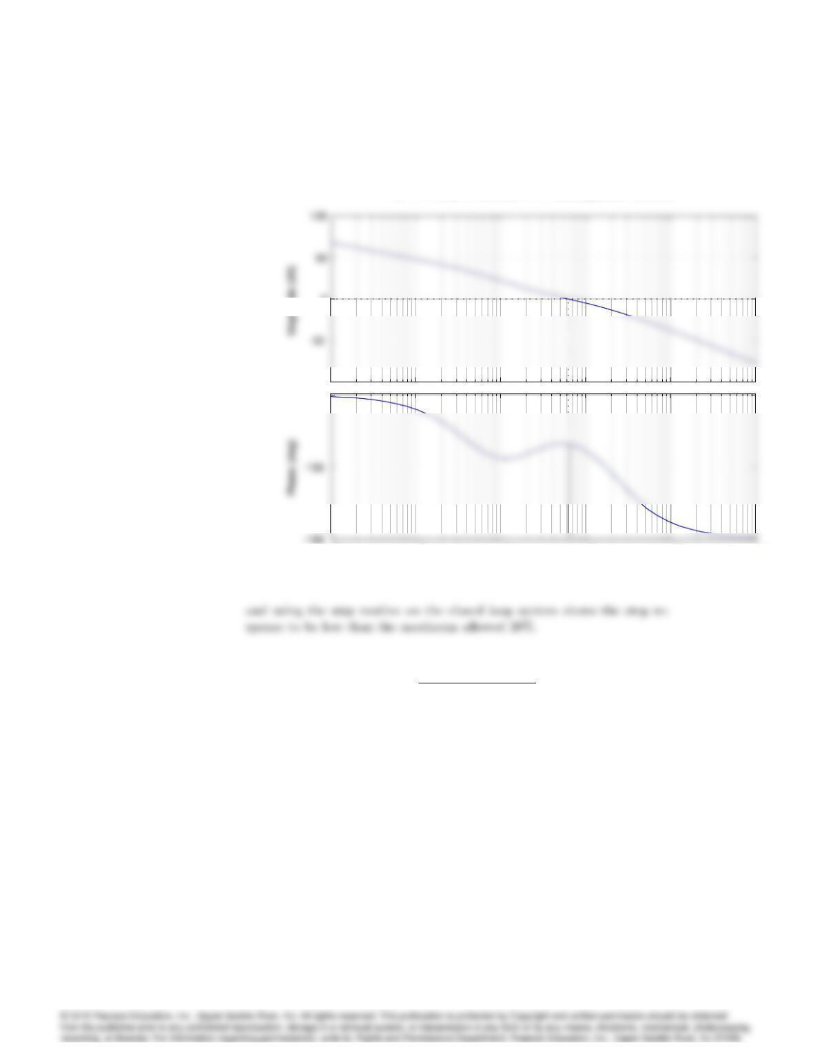
6138 CHAPTER 6. THE FREQUENCY-RESPONSE DESIGN METHOD
–100
0
10
-1
10
0
10
1
10
2
10
3
10
4
–90
Bode Diagram
Gm = Inf dB (at Inf rad/sec) , Pm = 59.5 deg (at 62.4 rad/sec)
Frequency (rad/sec)
–100
0
10
-1
10
0
10
1
10
2
10
3
10
4
–90
52. The open-loop transfer function of a unity feedback system is
G(s) = K
s(1 + s=5)(1 + s=20):
(a) Sketch the system block diagram including input reference commands
and sensor noise.
(b) Design a compensator for G(s)using Bode plot sketches so that the
closed-loop system satisfies the following specifications:
i. The steady-state error to a unit ramp input is less than 0.01.
ii. PM 45
iii. The steady-state error for sinusoidal inputs with ! < 0:2rad/sec
is less than 1/250.
iv. Noise components introduced with the sensor signal at frequen-
cies greater than 200 rad/sec are to be attenuated at the output
by at least a factor of 100,.
6139
(c) Verify and/or refine your design using Matlab including a compu-
tation of the closed-loop frequency response to verify (iv).
Solution :
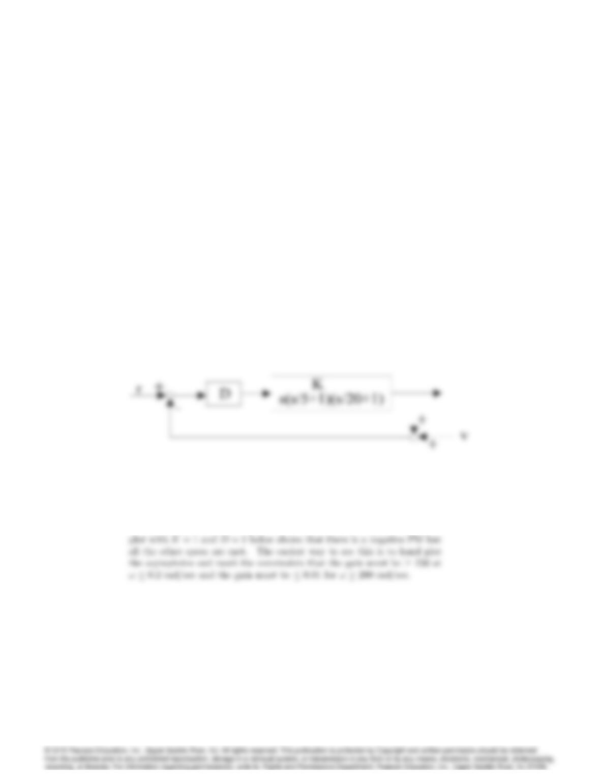
a. The block diagram shows the noise, v, entering where the sensor would
be:
b. The first specification implies Kv100 and thus K100:The bode