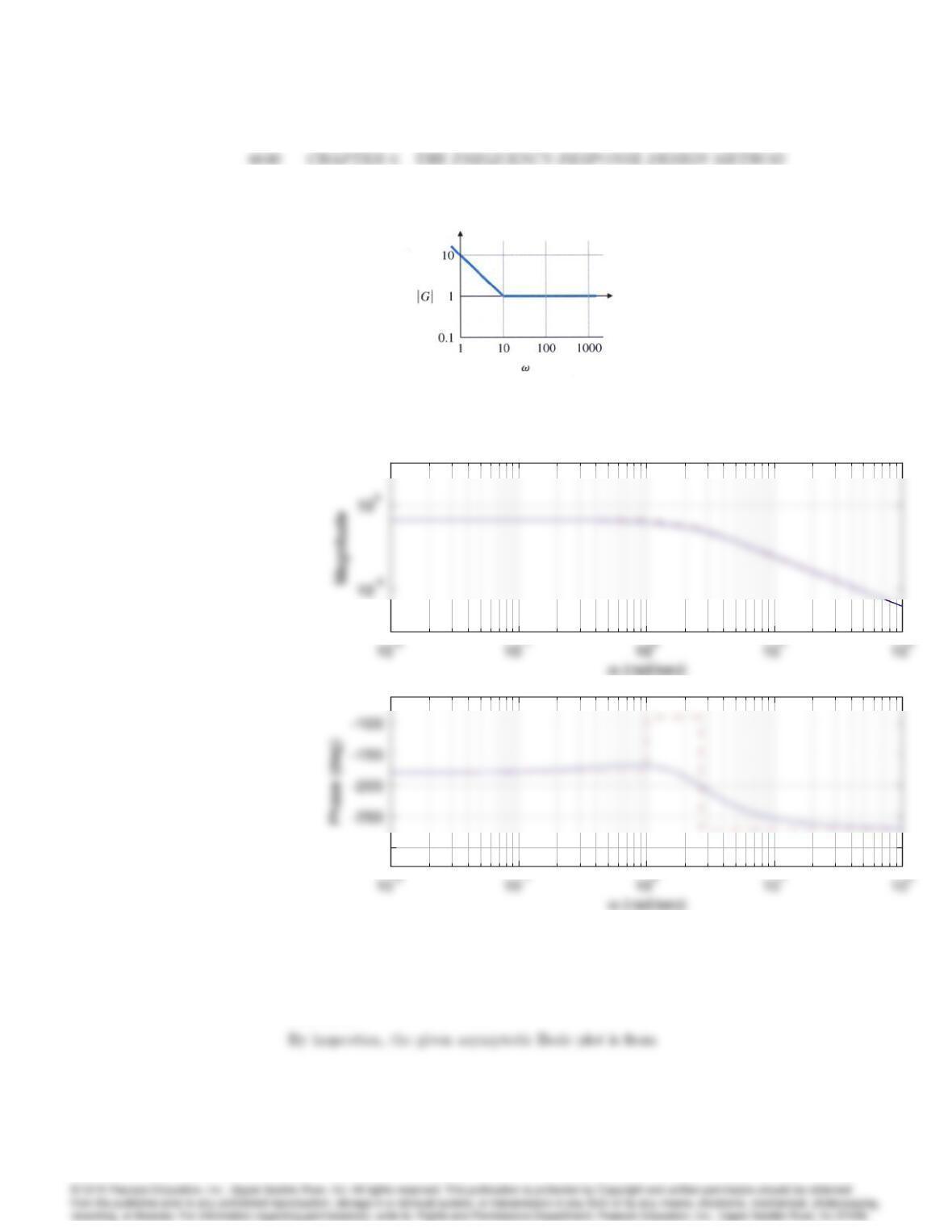
Figure 6.85: Magnitude portion of Bode plot for Problem 9
Bode plot for Prob. 6.8 (f)
Bode plot for Prob. 6.8 (f)
-300
Bode plot for Prob. 6.8 (f)
Bode plot for Prob. 6.8 (f)
-300
9. A certain system is represented by the asymptotic Bode diagram shown
in Fig. 6.85. Find and sketch the response of this system to a unit step
input (assuming zero initial conditions).
Solution:
6041
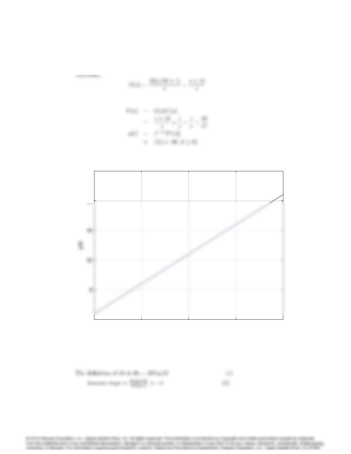
The response to a unit step input is :
00.5 11.5 2
0
20
25
Time (sec)
Prob. 6.9: Unit Step Response
00.5 11.5 2
0
20
25
Time (sec)
Prob. 6.9: Unit Step Response
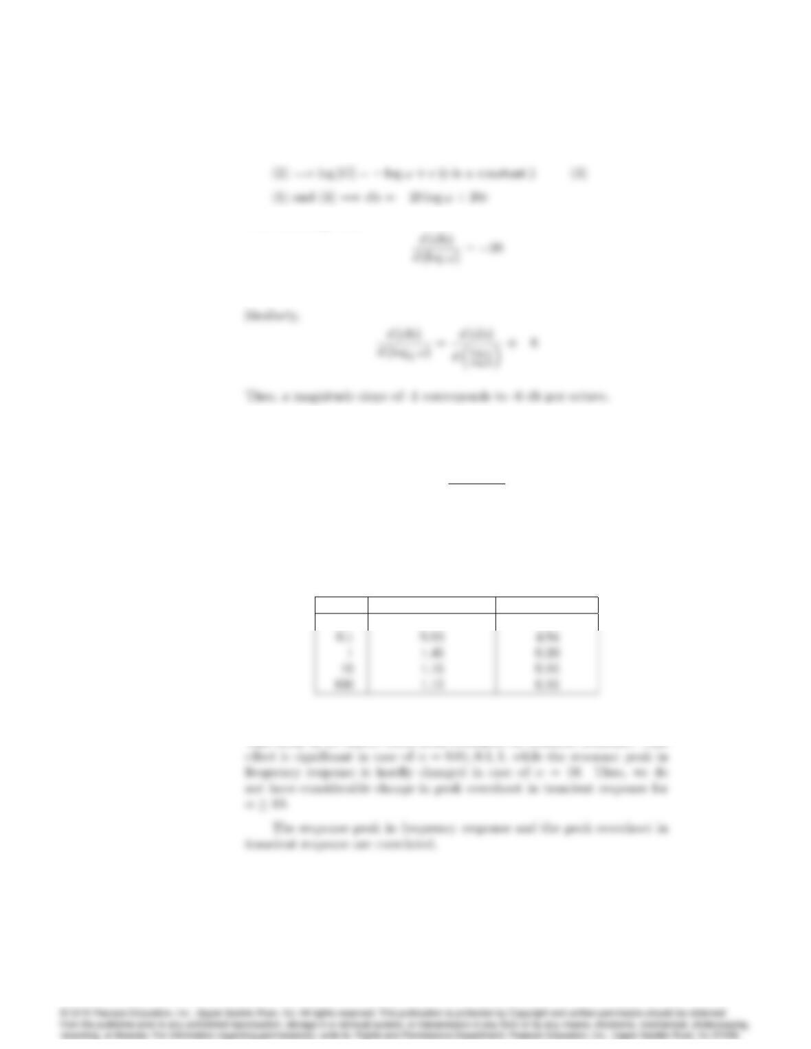
10. Prove that a magnitude slope of 1 in a Bode plot corresponds to 20 db
per decade or -6 db per octave.
Solution:
6042 CHAPTER 6. THE FREQUENCY-RESPONSE DESIGN METHOD
Differentiating this,
Thus, a magnitude slope of -1 corresponds to -20 db per decade.
11. A normalized second-order system with a damping ratio = 0:5and an
additional zero is given by
G(s) = s=a + 1
s2+s+ 1:
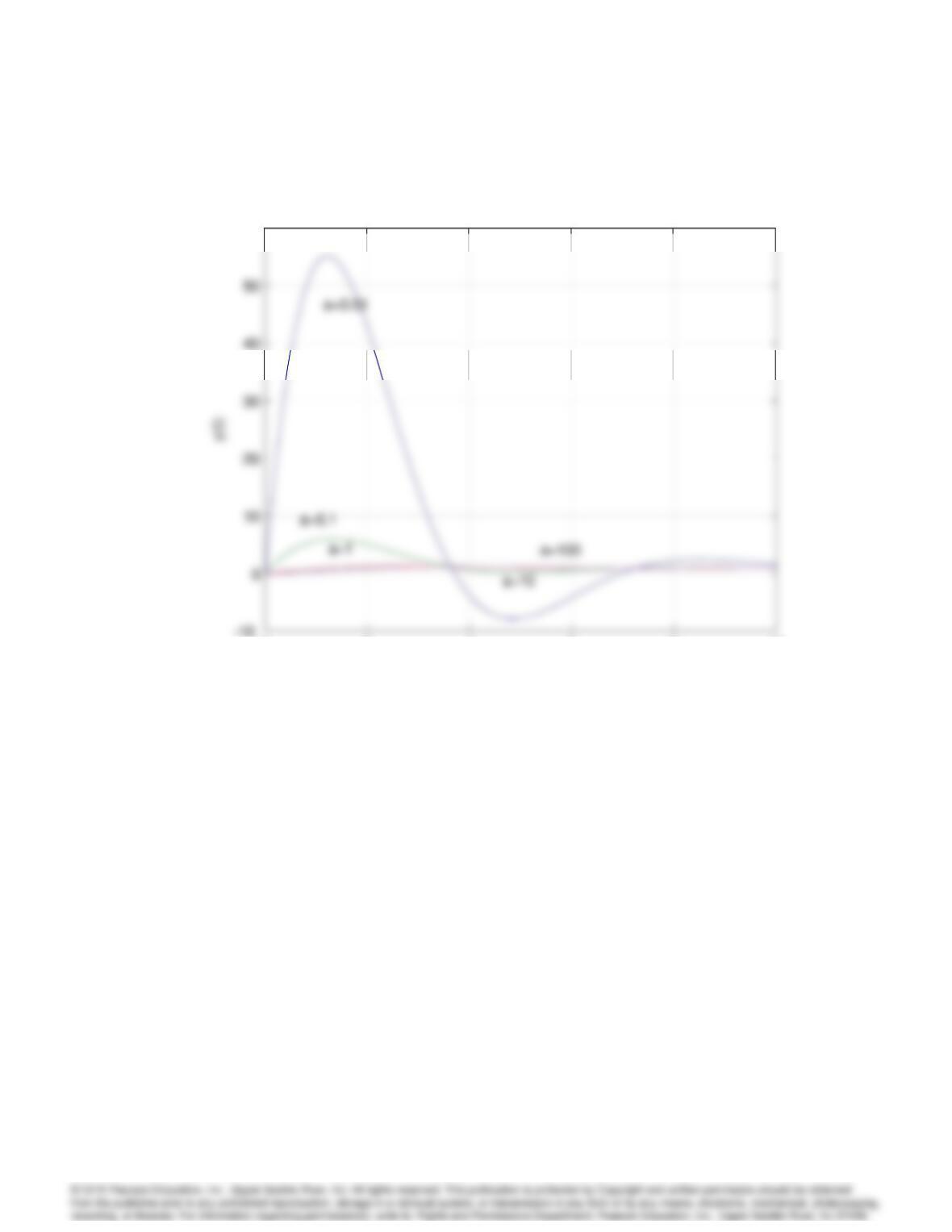
Use MATLAB to compare the Mpfrom the step response of the system
for a= 0:01;0:1, 1, 10, and 100 with the Mrfrom the frequency response
of each case. Is there a correlation between Mrand Mp?
Solution:
Resonant peak, MrOvershoot, Mp
0:01
98:8
54:1
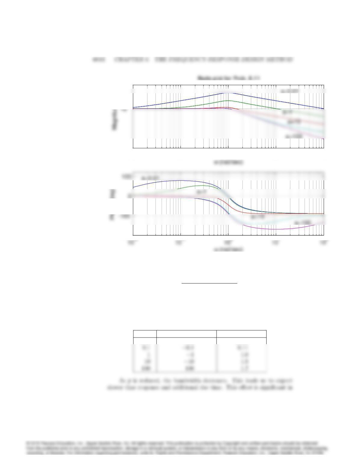
As is reduced, the resonant peak in frequency response increases.
This leads us to expect extra peak overshoot in transient response. This
6043
0 2 4 6 8 10
-10
60
Time (sec)
Unit Step Response
0 2 4 6 8 10
-10
60
Time (sec)
Unit Step Response
10-2 10-1 100101102
10-5
10-2 10-1 100101102
10-5
-200
10-2 10-1 100101102
10-5
10-2 10-1 100101102
10-5
a=0.1
-200
a=0.1
12. A normalized second-order system with = 0:5and an additional pole is
given by.
G(s) = 1
[(s=p) + 1](s2+s+ 1)
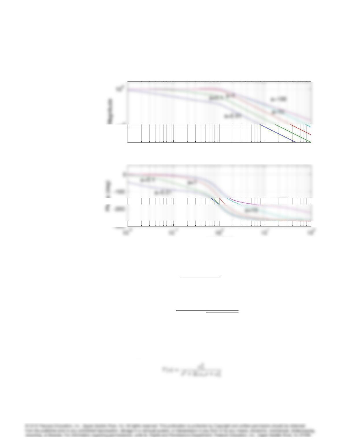
Draw Bode plots with p= 0:01;0:1, 1, 10 and 100. What conclusions can
you draw about the effect of an extra pole on the bandwidth compared to
the bandwidth for the second-order system with no extra pole?
Solution:
pAdditional pole (p) Bandwidth, !Bw
0:01
0:01
0:013
6045
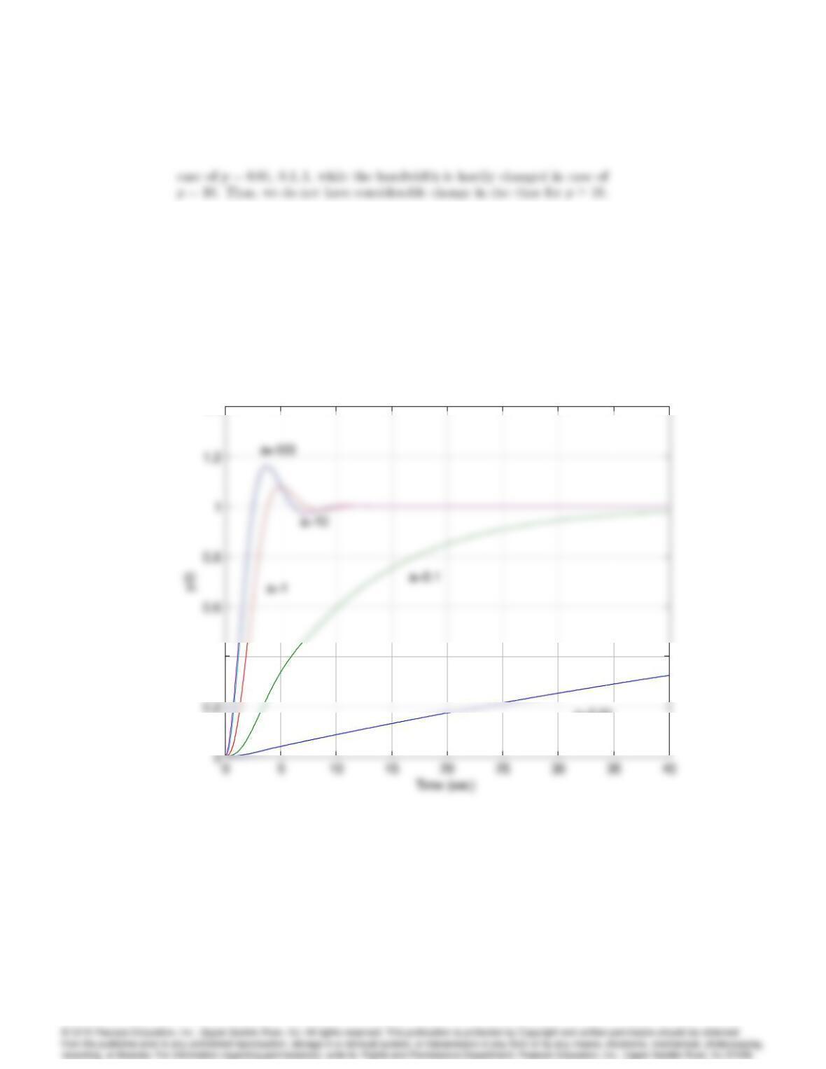
Bandwidth is a measure of the speed of response of a system, such as
rise time.
0.4
1.4
Unit Step Response
0.4
1.4
Unit Step Response
a=0.01
6046 CHAPTER 6. THE FREQUENCY-RESPONSE DESIGN METHOD
10-2 10-1 100101102
10-5
Frequency (rad/sec)
Magnitude
Bode plot for Prob. 6.12
10-2 10-1 100101102
10-5
Frequency (rad/sec)
Magnitude
Bode plot for Prob. 6.12
ω (rad/sec)
10-2 10-1 100101102
10-5
Frequency (rad/sec)
Magnitude
Bode plot for Prob. 6.12
10-2 10-1 100101102
10-5
Frequency (rad/sec)
Magnitude
Bode plot for Prob. 6.12
ω (rad/sec)
a=100
13. For the closed-loop transfer function
T(s) = !2
n
s2+ 2!ns+!2
n
;
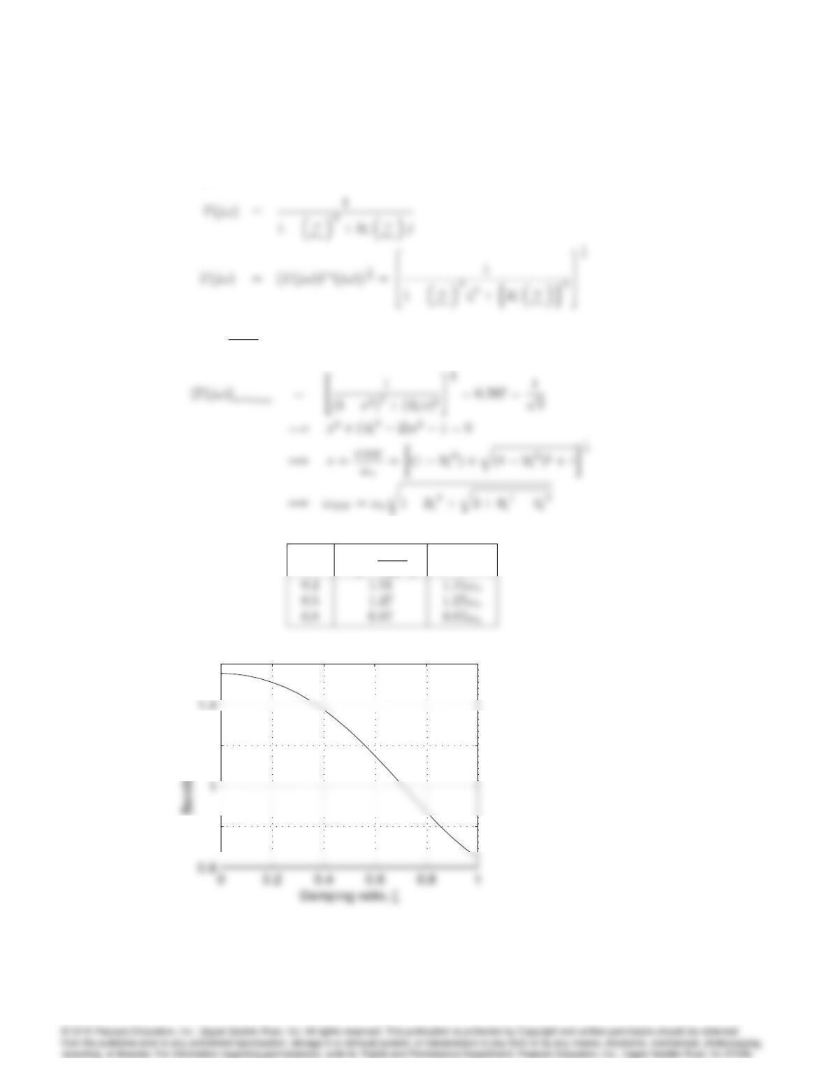
derive the following expression for the bandwidth !BW of T(s)in terms
of !nand :
!BW =!nr122+q2 + 4442:
Assuming !n= 1, plot !BW for 01.
Solution :
The closed-loop transfer function :
6047
s=j!;
Let x=!BW
!n
:
x =!BW
!n!BW
0.8
1.2
1.6
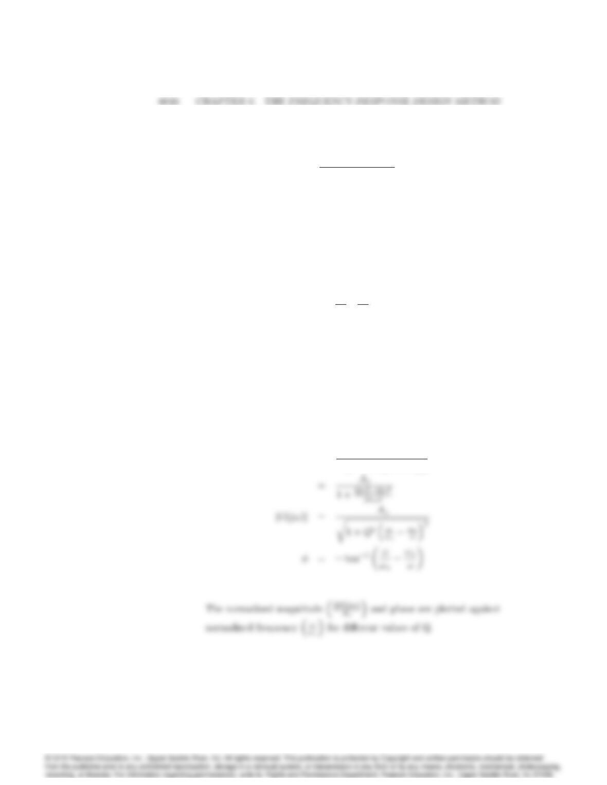
Bandwidth vs zeta
14. Consider the system whose transfer function is
G(s) = A0!0s
Qs2+!0s+!2
0Q:
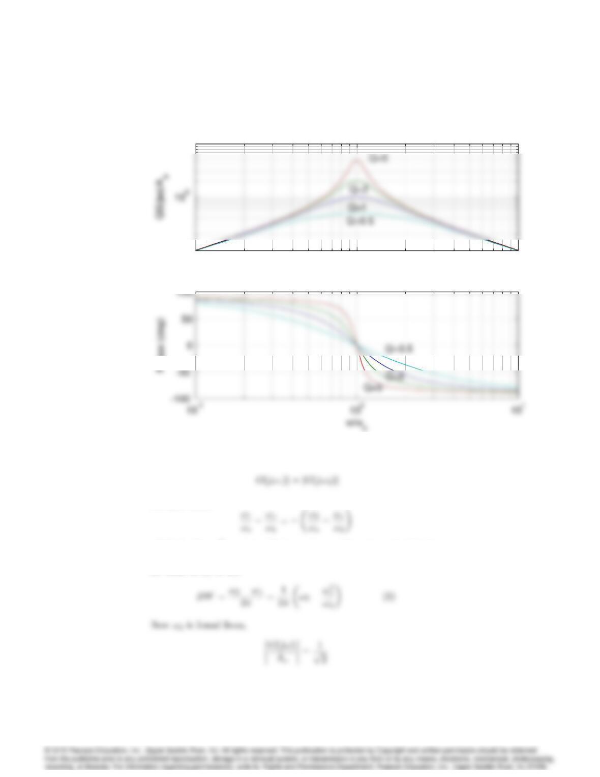
This is a model of a tuned circuit with quality factor Q. (a) Compute the
magnitude and phase of the transfer function analytically, and plot them
for Q= 0:5, 1, 2, and 5 as a function of the normalized frequency !=!0.
(b) Define the bandwidth as the distance between the frequencies on either
side of !0where the magnitude drops to 3 db below its value at !0and
show that the bandwidth is given by
BW =1
2!0
Q:
(c) What is the relation between Q and ?
Solution :
(a) Let s=j!;
G(j!) = Ao!oj!
Q!2+!oj! +!2
oQ
6049
10-1 100101
10-1
101
ω/ωo
Bode plot for Prob. 6.14
10-1 100101
10-1
101
ω/ωo
Bode plot for Prob. 6.14
10-1 100101
10-1
101
ω/ωo
Bode plot for Prob. 6.14
10-1 100101
10-1
101
ω/ωo
Bode plot for Prob. 6.14
Q=1
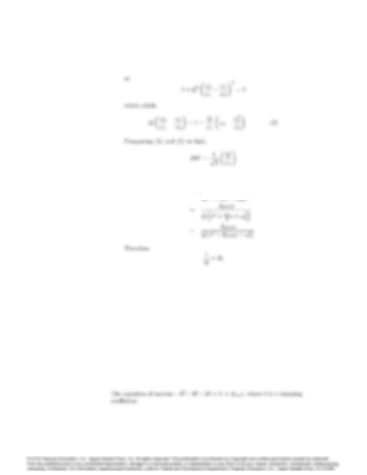
(b) There is symmetry around !o. For every frequency !1< !o, there
exists a frequency !2> !owhich has the same magnitude
We have that,
which implies !2
o=!1!2. Let !1< !oand !2> !obe the two
frequencies on either side of !ofor which the gain drops by 3db from
its value of Aoat !o.
6050 CHAPTER 6. THE FREQUENCY-RESPONSE DESIGN METHOD
(c)
G(s) = A0!0s
Qs2+!0s+!2
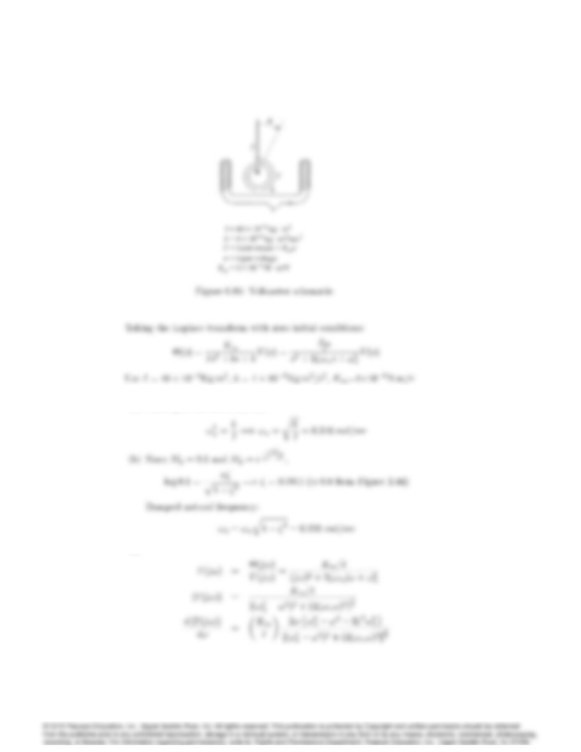
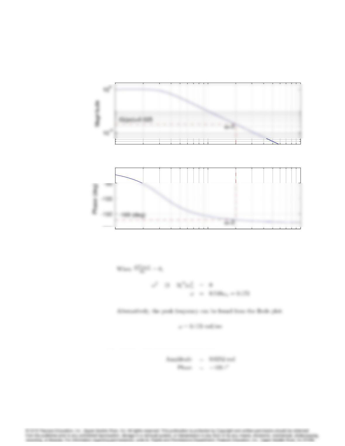
15. A DC voltmeter schematic is shown in Fig. 6.86. The pointer is damped
so that its maximum overshoot to a step input is 10%.
(a) What is the undamped natural frequency of the system?
(b) What is the damped natural frequency of the system?
(c) Plot the frequency response using MATLAB to determine what input
frequency will produce the largest magnitude output?
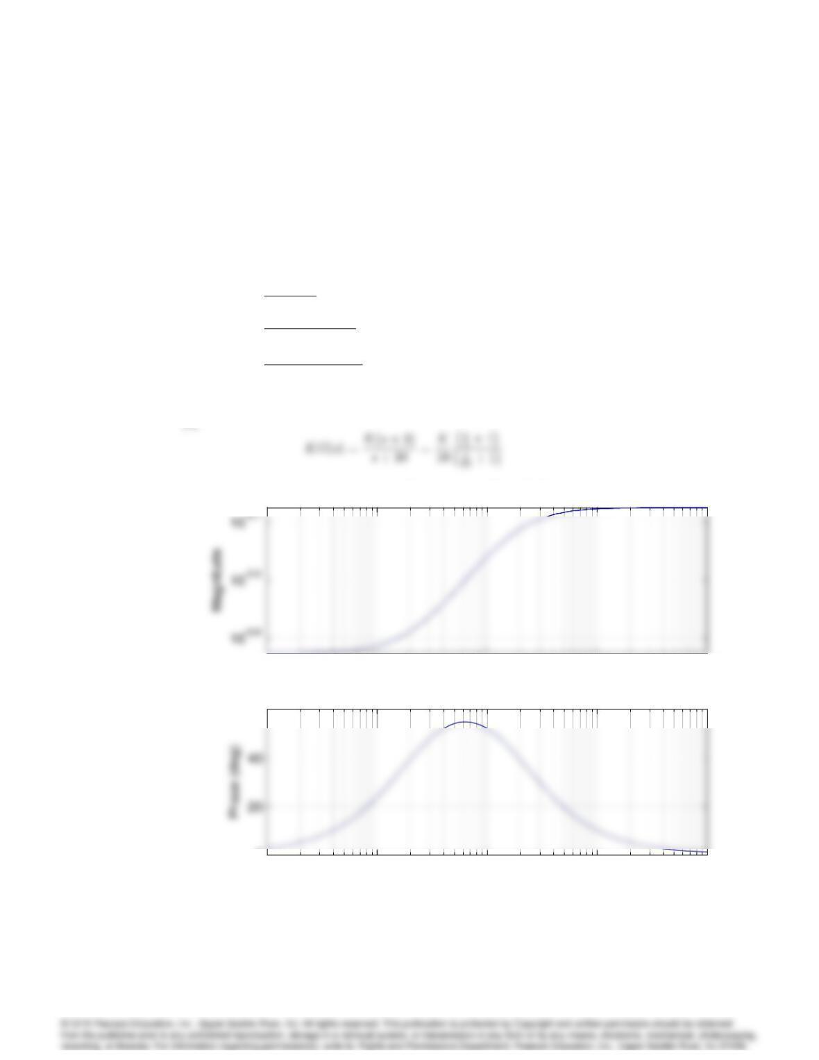
(d) Suppose this meter is now used to measure a 1-V AC input with a
frequency of 2 rad/sec. What amplitude will the meter indicate after
initial transients have died out? What is the phase lag of the output
with respect to the input? Use a Bode plot analysis to answer these
questions. Use the lsim command in MATLAB to verify your answer
in part (d).
Solution :
6051
(a) Undamped natural frequency:
(c)
6052 CHAPTER 6. THE FREQUENCY-RESPONSE DESIGN METHOD
10-1 100101
ω (rad/sec)
Bode plot for Prob. 6.15
10-1 100101
ω (rad/sec)
Bode plot for Prob. 6.15
10-1 100101
-200
0
ω (rad/sec)
10-1 100101
ω (rad/sec)
Bode plot for Prob. 6.15
10-1 100101
ω (rad/sec)
Bode plot for Prob. 6.15
10-1 100101
-200
0
ω (rad/sec)
(d) With != 2 rad/sec from the Bode plot:
6053
Problems and Solutions for Section 6.2
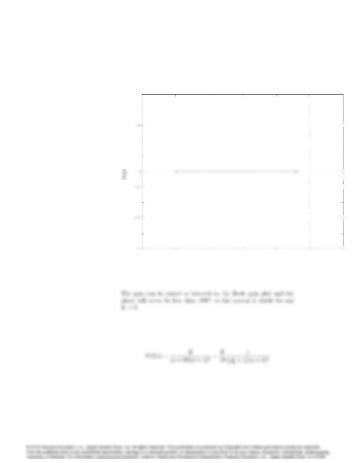
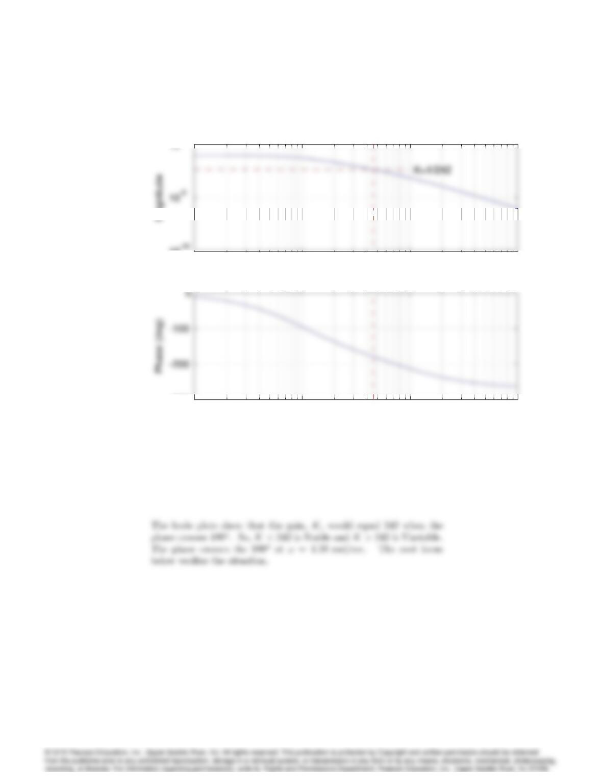
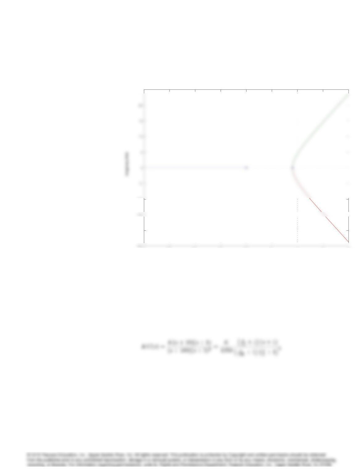
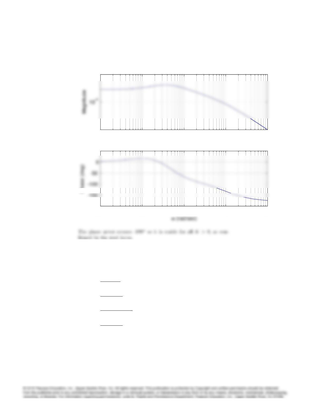
16. Determine the range of Kfor which the closed-loop systems (see Fig. 6.18)
are stable for each of the cases below by making a Bode plot for K= 1 and
imagining the magnitude plot sliding up or down until instability results.
Verify your answers using a very rough sketch of a root-locus plot.
(a) KG(s) = K(s+ 3)
s+ 30
(b) KG(s) = K
(s+ 10)(s+ 1)2
(c) KG(s) = K(s+ 10)(s+ 1)
(s+ 100)(s+ 5)3
Solution :
(a)
10-1 100101102103
ω (rad/sec)
Bode plot for Prob. 6.16 (a)
10-1 100101102103
ω (rad/sec)
Bode plot for Prob. 6.16 (a)
10-1 100101102103
0
60
ω (rad/sec)
10-1 100101102103
ω (rad/sec)
Bode plot for Prob. 6.16 (a)
10-1 100101102103
ω (rad/sec)
Bode plot for Prob. 6.16 (a)
10-1 100101102103
0
60
ω (rad/sec)
6054 CHAPTER 6. THE FREQUENCY-RESPONSE DESIGN METHOD
-25 -20 -15 -10 -5 0 5
–0.8
–0.4
0.2
0.4
0.8
1
Root Locus
Real Axis
(b)
6055
10-1 100101102
10-10
ω (rad/sec)
Bode plot for Prob. 6.16(b)
10-1 100101102
10-10
ω (rad/sec)
Bode plot for Prob. 6.16(b)
10-1 100101102
-300
ω (rad/sec)
10-1 100101102
10-10
ω (rad/sec)
Bode plot for Prob. 6.16(b)
10-1 100101102
10-10
ω (rad/sec)
Bode plot for Prob. 6.16(b)
10-1 100101102
-300
ω (rad/sec)
6056 CHAPTER 6. THE FREQUENCY-RESPONSE DESIGN METHOD
-30 -25 -20 -15 -10 -5 0 5 10
-20
-10
25
Root Locus
Real Axis
(c)
6057
10-1 100101102103
10-6
10-2
ω (rad/sec)
Bode plot for Prob. 6.16 (c)
10-1 100101102103
10-6
10-2
ω (rad/sec)
Bode plot for Prob. 6.16 (c)
10-1 100101102103
-200
50
Phase (deg)
10-1 100101102103
10-6
10-2
ω (rad/sec)
Bode plot for Prob. 6.16 (c)
10-1 100101102103
10-6
10-2
ω (rad/sec)
Bode plot for Prob. 6.16 (c)
10-1 100101102103
-200
50
Phase (deg)
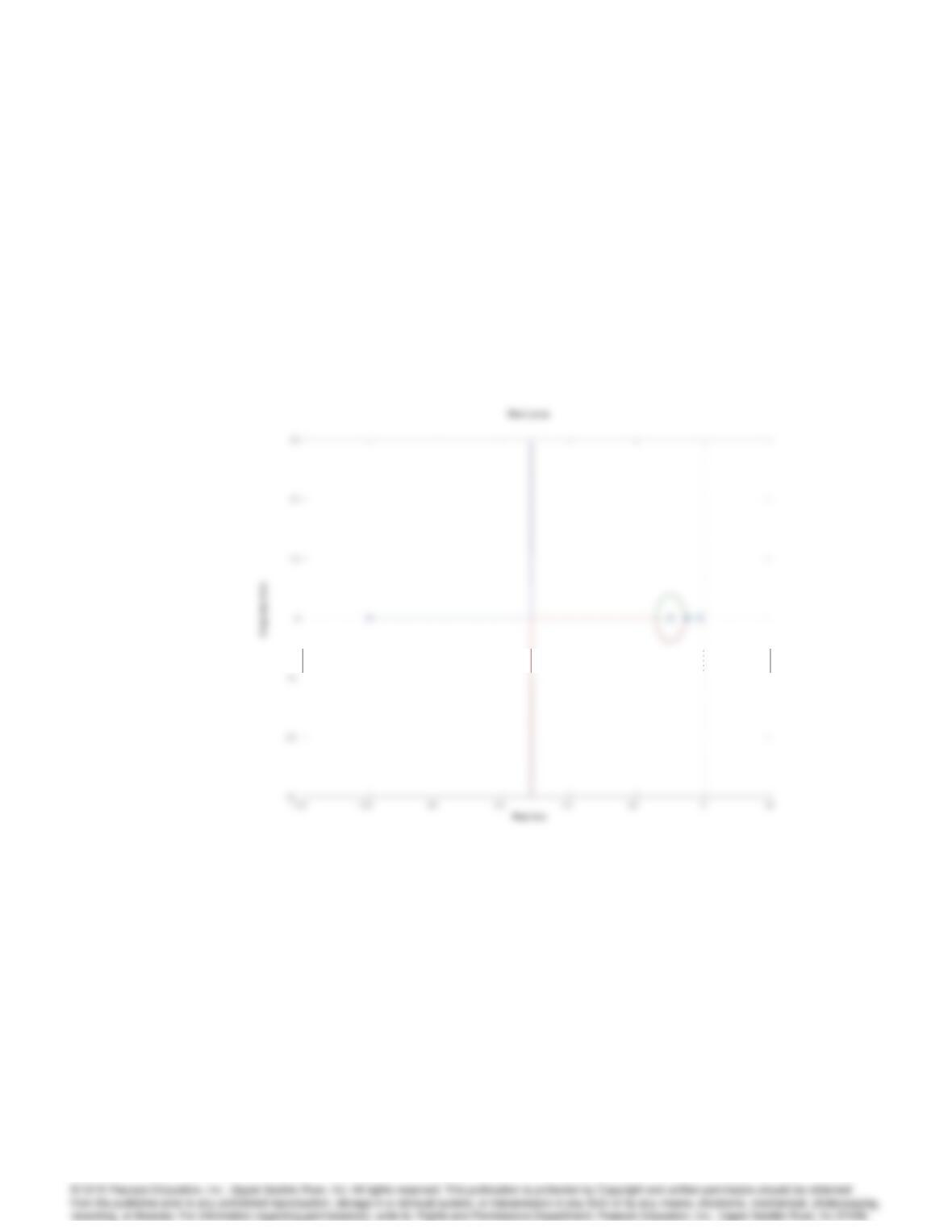
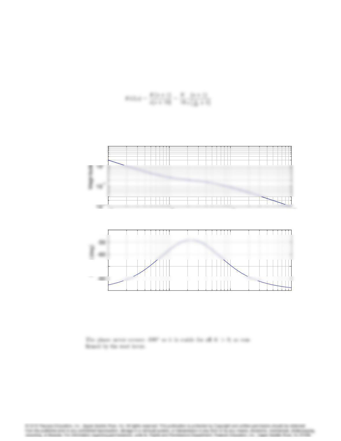
17. Determine the range of Kfor which each of the following systems is stable
by making a Bode plot for K= 1 and imagining the magnitude plot
sliding up or down until instability results. Verify your answers using a
very rough sketch of a root-locus plot.
(a) KG(s) = K(s+ 1)
s(s+ 10)
(b) KG(s) = K(s+ 1)
s2(s+ 10)
(c) KG(s) = K
(s+ 2)(s2+ 9)
(d) KG(s) = K(s+ 1)2
s3(s+ 10)
Solution :
6058 CHAPTER 6. THE FREQUENCY-RESPONSE DESIGN METHOD
6059
(a)
10-1 100101102
101
ω (rad/sec)
Bode plot for Prob. 6.17 (a)
10-1 100101102
101
ω (rad/sec)
Bode plot for Prob. 6.17 (a)
10-1 100101102
-90
-70
-40
ω (rad/sec)
Phase (deg)
10-1 100101102
101
ω (rad/sec)
Bode plot for Prob. 6.17 (a)
10-1 100101102
101
ω (rad/sec)
Bode plot for Prob. 6.17 (a)
10-1 100101102
-90
-70
-40
ω (rad/sec)
Phase (deg)