25. Assume that the unity feedback system of Fig. 5.53 has the open-loop
plant
G(s) = 1
s(s+ 3)(s+ 6):
Design a lag compensation to meet the following specifications:
The step response settling time is to be less than 5 sec.
The step response overshoot is to be less than 17%.
The steady-state error to a unit ramp input must not exceed 10%.
Solution:
The overshoot specification requires that damping be 0:5and the
R oot Locus
4
6
0. 965
0. 92
0. 99
0.4
0.8
1.2
1.4
Root locus and step response for Problem 5.25
5041
26. A numerically controlled machine tool positioning servomechanism has a
normalized and scaled transfer function given by
G(s) = 1
s(s+ 1):
Performance specifications of the system in the unity feedback configu-
ration of Fig. 5.53 are satisfied if the closed-loop poles are located at
s=1jp3.
(a) Show that this specification cannot be achieved by choosing propor-
tional control alone, Dc(s) = kp.
(b) Design a lead compensator Dc(s) = Ks+z
s+pthat will meet the speci-
fication.
Solution:
27. A servomechanism position control has the plant transfer function
G(s) = 10
s(s+ 1)(s+ 10):
You are to design a series compensation transfer function Dc(s)in the
unity feedback configuration to meet the following closed-loop specifica-
tions:
The response to a reference step input is to have no more than 16%
overshoot.
The response to a reference step input is to have a rise time of no
more than 0.4 sec.
The steady-state error to a unit ramp at the reference input must be
less than 0.05.
(a) Design a lead compensation that will cause the system to meet the
dynamic response specifications, ignoring the error requirement.
(b) What is the velocity constant Kvfor your design? Does it meet the
error specification?
(c) Design a lag compensation to be used in series with the lead you
have designed to cause the system to meet the steady-state error
specification.
(d) Give the Matlab plot of the root locus of your final design.
(e) Give the Matlab response of your final design to a reference step.
Solution:
(a) Setting the lead pole at p=60 and the zero at z=1;the dynamic
(b)
5043
-10 -8 -6 -4 -2 0 2
-3
-2
-1
2
0.965
0.99
0.965
0.99
Lead root locus
Real Axis
00.5 11.5
0.5
1
Lead Step respons e
Time (sec)
-10 -8 -6 -4 -2 0 2
-3
-1
3
4
0.84
0.92
0.99
0.220.420.60.740.84
0.92
0.99
0.220.420.60.74
Lead-lag root locus
Real Axis
0 1 2 3 4 5 6 7
0
0.5
1.5
Lead-lag step response
Time (sec)
Solution to Problem 5.27

5044 CHAPTER 5. THE ROOT-LOCUS DESIGN METHOD
28. Assume the closed-loop system of Fig. 5.53 has a feed forward transfer
function G(s)given by
G(s) = 1
s(s+ 2):
Design a lag compensation so that the dominant poles of the closed-loop
system are located at s=1jand the steady-state error to a unit ramp
input is less than 0.2.
Solution:
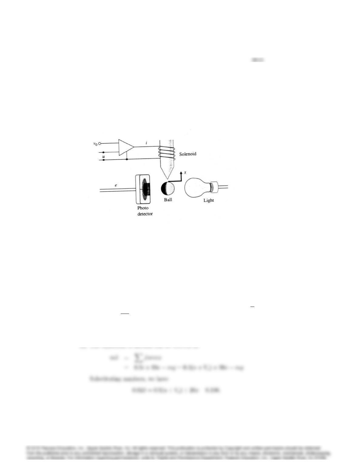
29. An elementary magnetic suspension scheme is depicted in Fig. 5.54. For
small motions near the reference position, the voltage eon the photo
detector is related to the ball displacement x(in meters) by e= 100x.
The upward force (in newtons) on the ball caused by the current i(in
amperes) may be approximated by f= 0:5i+ 20x. The mass of the ball
is 20 g, and the gravitational force is 9.8 N/kg. The power amplifier is a
voltage-to-current device with an output (in amperes) of i=u+V0.
Figure 5.54: Elementary magnetic suspension
(a) Write the equations of motion for this setup.
(b) Give the value of the bias V0that results in the ball being in equilib-
rium at x= 0.
(c) What is the transfer function from uto e?
(d) Suppose the control input uis given by u=Ke. Sketch the root
locus of the closed-loop system as a function of K.
(e) Assume that a lead compensation is available in the form U
E=
Dc(s) = Ks+z
s+p:Give values of K; z; and pthat yields improved
performance over the one proposed in part (d).
Solution:
(a) The equations of motion can be written as
5046 CHAPTER 5. THE ROOT-LOCUS DESIGN METHOD
(c) Taking Laplace transforms of the equation and substituting e= 100x;
(d) The locus starts at the two poles symmetric to the imaginary axis,
meet at the origin and cover the imaginary axis. The locus is plotted
below.
–40 – 30 –20 –10 010 20 30 40
–40
–20
40
Root Locus
Real Axis
Root loci for Problem 5.29d
(e) Since the system with a proportional gain is on the stability bound-
5047
–160 –140 – 120 –100 –80 – 60 –40 – 20 020 40
–40
–20
–10
40
50
Root Locus
Real Axis
Root loci for Problem 5.29e
30. A certain plant with the non minimum phase transfer function
G(s) = 42s
s2+s+ 9;
is in a unity positive feedback system with the controller transfer function
Dc(s):
(a) Use Matlab to determine a (negative) value for Dc(s) = Kso that
the closed-loop system with negative feedback has a damping ratio
= 0:707.
(b) Use Matlab to plot the system’s response to a reference step.
Solution:
(a) With all the negatives, the problem statement might be confusing.
(b) The final value of the step response plotted below is 0:887. To get
a positive output we would use a positive gain in positive feedback.
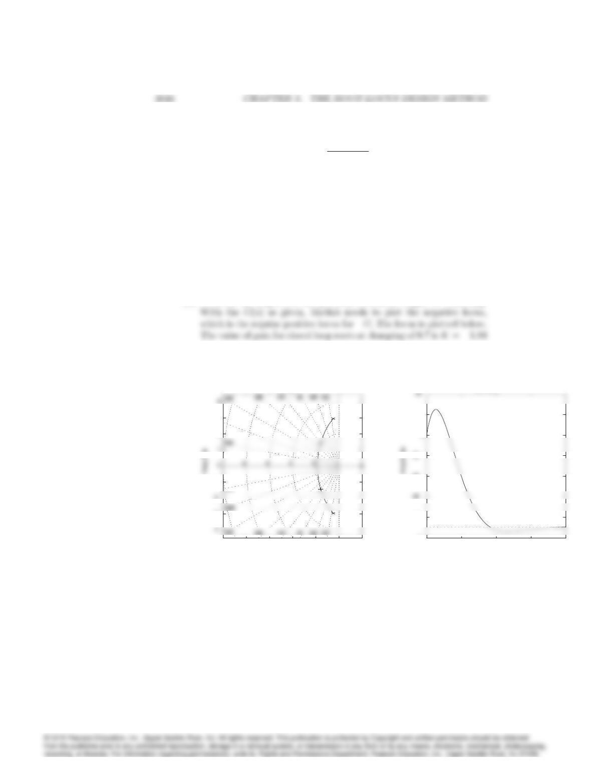
Root Locus
Real Axis
– 10 -8 -6 -4 -2 0 2
-3
-2
-1
2
3
0.99
0.965
St e p Res po ns e
Ti me ( sec)
0 1 2 3 4
-1
–0.8
–0.4
–0.2
0
0.2
Solutions for Problem 5.30
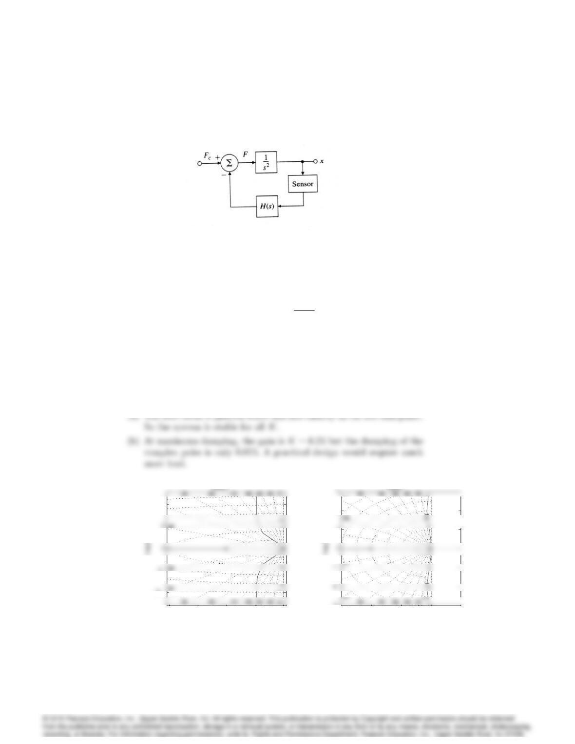
5049
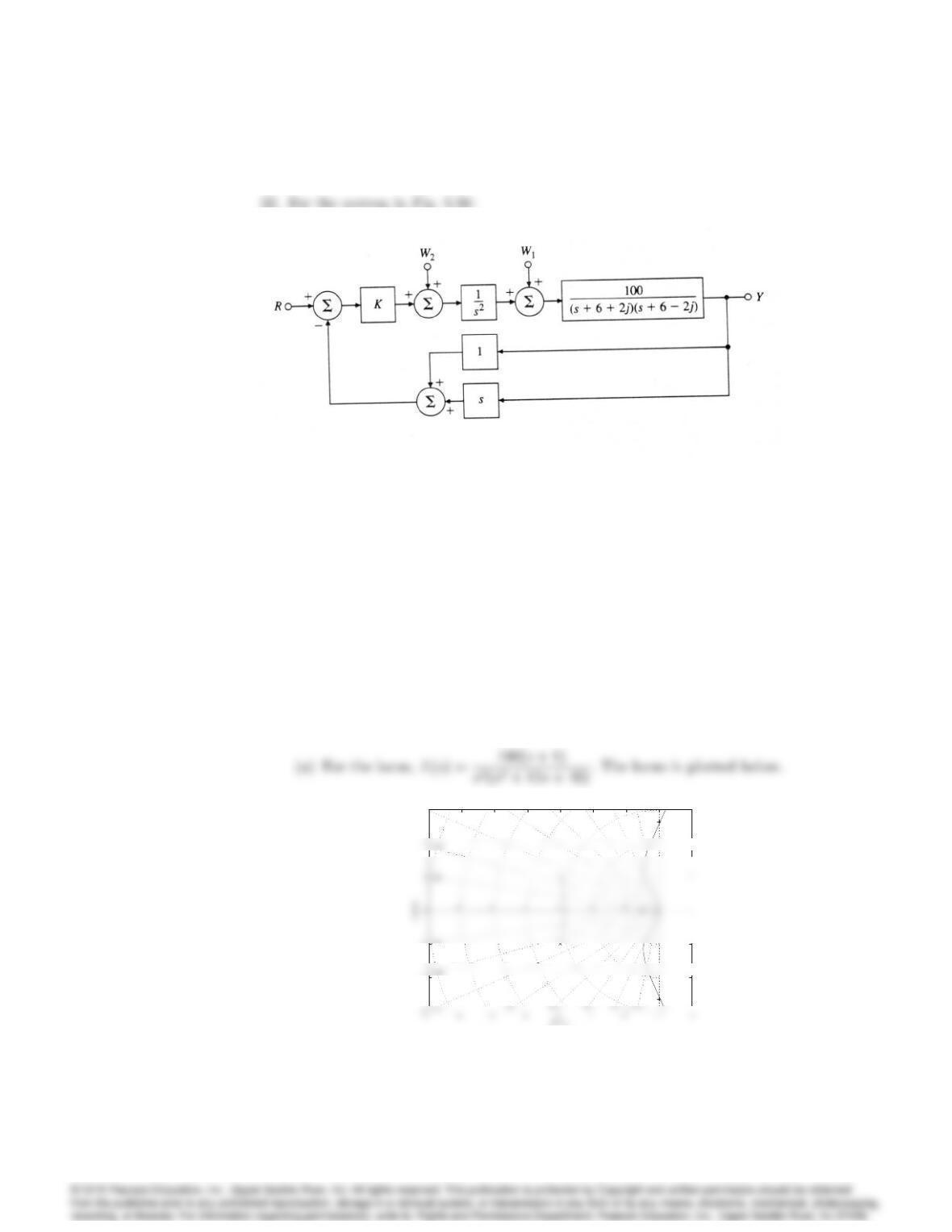
31. Consider the rocket-positioning system shown in Fig. 5.55.
Figure 5.55: Block diagram for rocket-positioning control system
(a) Show that if the sensor that measures xhas a unity transfer function,
the lead compensator
H(s) = Ks+ 2
s+ 4
stabilizes the system.
(b) Assume that the sensor transfer function is modeled by a single pole
with a 0:1sec time constant and unity DC gain. Using the root-locus
procedure, find a value for the gain Kthat will provide the maximum
damping ratio.
Solution:
Real Axis
-4 -3 -2 -1 0
–10
-5
10
10
6
2
10
8
4
2
0. 65
0.4
Real Axis
-3 -2 -1 0 1
-3
1
2
3
1.5
0.5
2.5
2
1
0.5
0. 88
0. 97
0. 76
Loci for Problem 5.31
5050 CHAPTER 5. THE ROOT-LOCUS DESIGN METHOD
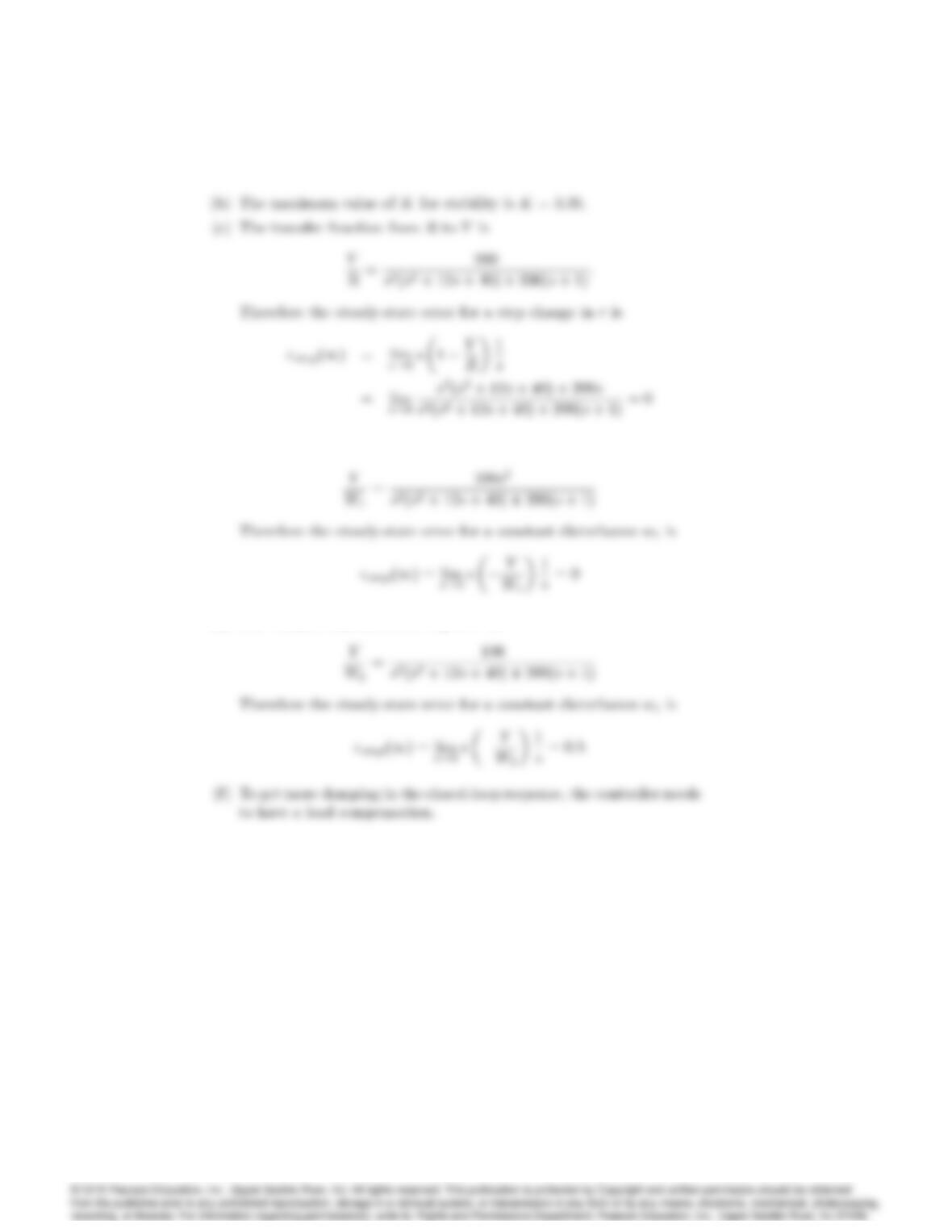
Figure 5.56: Control system for Problem 5.32
(a) Find the locus of closed-loop roots with respect to K.
(b) Find the maximum value of Kfor which the system is stable. Assume
K= 2 for the remaining parts of this problem.
(c) What is the steady-state error (e=ry) for a step change in r?
(d) What is the steady-state error in yfor a constant disturbance w1?
(e) What is the steady-state error in yfor a constant disturbance w2?
(f) If you wished to have more damping, what changes would you make
to the system?
Solution:
Root Locus
-4
-2
6
0.99
0.92 0.84 0.74 0.6 0.42 0.22
Locus for Problem 5.32
5051
(d) The transfer function from W1to Yis:
(e) The transfer function from W2to Yis:
33. Consider the plant transfer function
G(s) = bs +k
s2[mMs2+ (M+m)bs + (M+m)k]
to be put in the unity feedback loop of Fig. 5.53. This is the transfer
function relating the input force u(t)and the position y(t)of mass Min
the non-collocated sensor and actuator problem. In this problem, we will
use root-locus techniques to design a controller Dc(s)so that the closed-
loop step response has a rise time of less than 0.1 sec and an overshoot of
less than 10%. You may use Matlab for any of the following questions:
(a) Approximate G(s)by assuming that m
=0, and let M= 1,k= 1,
b= 0:1, and Dc(s) = K. Can Kbe chosen to satisfy the performance
specifications? Why or why not?
(b) Repeat part (a) assuming Dc(s) = K(s+z), and show that Kand z
can be chosen to meet the specifications.
(c) Repeat part (b) but with a practical controller given by the transfer
function
Dc(s) = Kp(s+z)
s+p;
and pick pso that the values for Kand zcomputed in part (b) remain
more or less valid.
(d) Now suppose that the small mass mis not negligible, but is given by
m=M=10. Check to see if the controller you designed in part (c)
still meets the given specifications. If not, adjust the controller pa-
rameters so that the specifications are met.
Solution:
(b) The specs require that > 0:6; !n>18:Select z= 15 for a start.
5053
-10
20
Root Locus
Real Ax is
1.5
-20
-10
20
Root Locus
Real Ax is
00.2 0.4 0.6 0.8 1
1.5
-10 -8 -6 -4 -2 0 2
-2
4
Root Locus
Real Ax is
00.5 11.5 22.5 33.5
1.5
Root loci and step responses for Problem 5.33
5054 CHAPTER 5. THE ROOT-LOCUS DESIGN METHOD
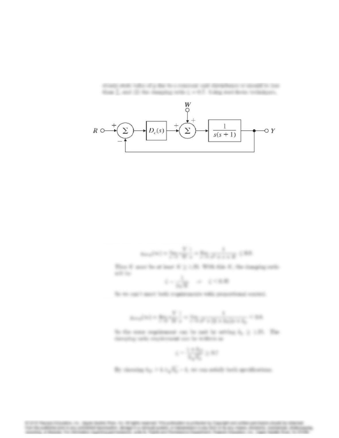
34. Consider the Type 1 system drawn in Fig. 5.57. We would like to de-
sign the compensation Dc(s)to meet the following requirements: (1) The
Figure 5.57: Control system for Problem 5.34
(a) Show that proportional control alone is not adequate.
(b) Show that proportional-derivative control will work.
(c) Find values of the gains kpand kDfor Dc(s) = kp+kDsthat meet
the design specifications with at least a 10% margin.
Solution:
(a) To meet the error requirement, we need
(b) With PD control,
5055
(c) Setting kp= 1:4and kD= 0:85, we get ystep(1) = 0:714 and =
1 .5
0.350.580.760.860.92
0.96
Root Locus
0 .1
0 .5
0 .8
Step response for problem 5.34
Solution for Problem 5.34
5056 CHAPTER 5. THE ROOT-LOCUS DESIGN METHOD
35. Using a sample rate of 10 Hz, find the Dc(z)that is the discrete equivalent
to your Dc(s)from Problem 5.34 using the trapezoid rule. Evaluate the
5.7 rather than the correct one, Problem 5.34)
Solution:
From Problem 5.34, we have Dc(s) = 0:85s+ 1:4. The discrete equivalent
0.2
Solution for Problem 5.35
Note that there is slightly greater overshoot in the digital system, which

5057
5058 CHAPTER 5. THE ROOT-LOCUS DESIGN METHOD
Problems and solutions for Section 5.5
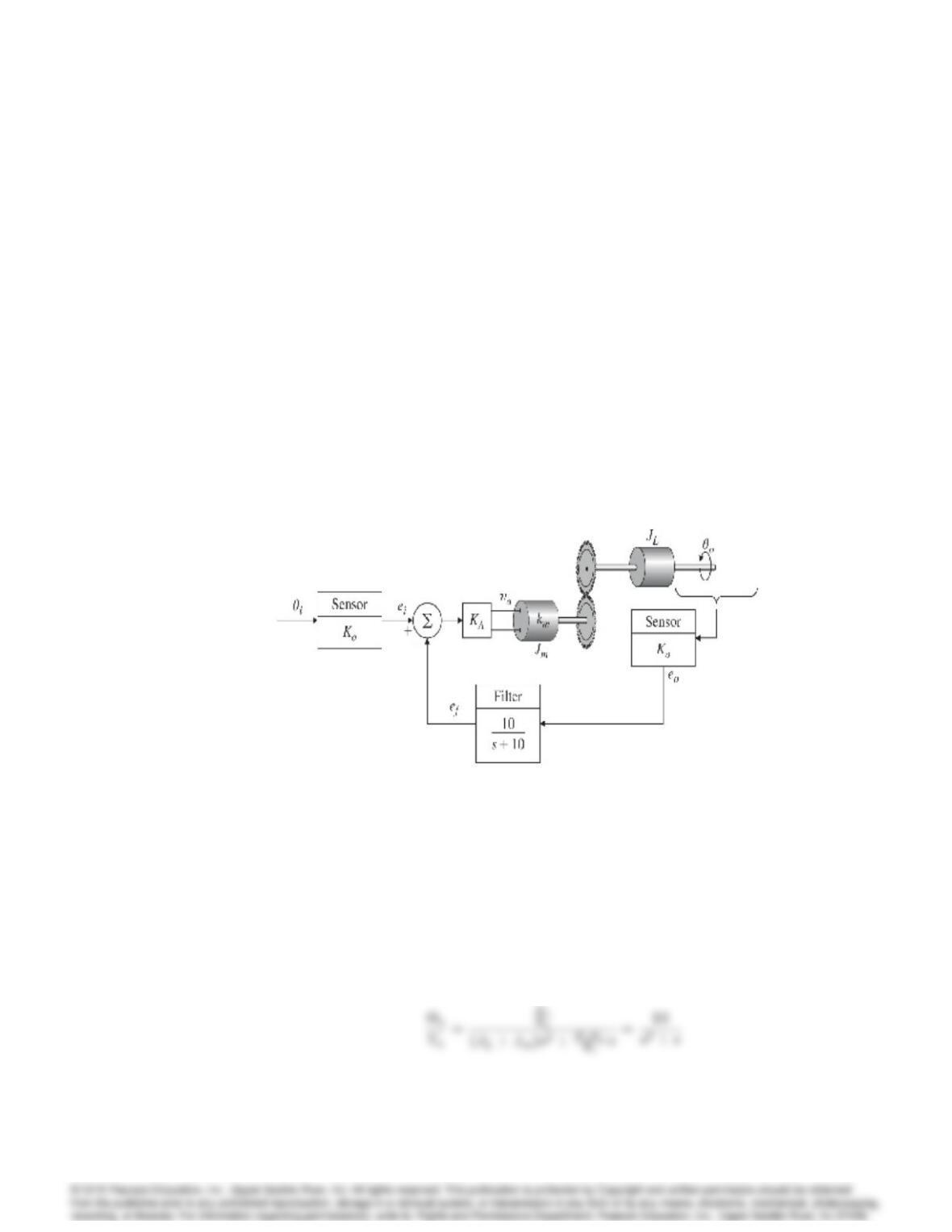
36. Consider the positioning servomechanism system shown in Fig. 5.58, where
ei=Koi; eo=Koo; Ko= 10V=rad;
(note: 1st printing of book had eo=Kpoto;which is not correct)
T= motor torque = Ktia;
km=Kt= torque constant = 0:1 N m=A;
Ke= back emf constant = 0:1V sec
Ra= armature resistance = 10;
Gear ratio = 1 : 1;
JL+Jm= total inertia = 103kg m2;
va=KA(eief):
Figure 5.58: Positioning servomechanism
(a) What is the range of the amplifier gain KAfor which the system is
stable? Estimate the upper limit graphically using a root-locus plot.
(b) Choose a gain KAthat gives roots at = 0:7. Where are all three
closed-loop root locations for this value of KA?
Solution:
(a) Neglecting viscous friction and the effect of inductance, the transfer
function of the DC motor is
5059
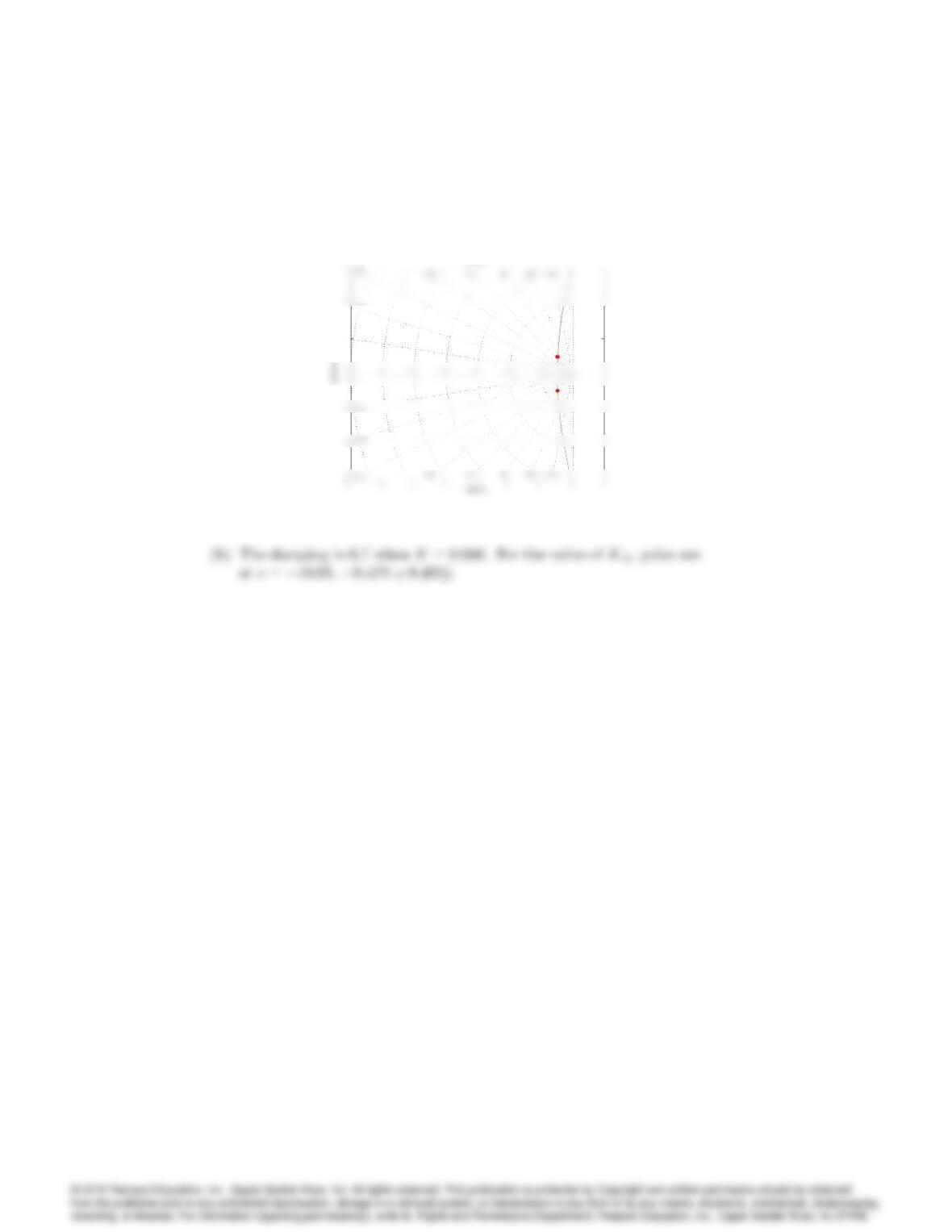
From the root locus plotted below, the upper limit of KAfor stability
is 0:11.
1
0.965
0.99
Root Loc us
Root locus for Problem 5.36