Operating Systems Chapter 5 Homework Using The Final Value Theorem The Steady state

5060 CHAPTER 5. THE ROOT-LOCUS DESIGN METHOD

37. We wish to design a velocity control for a tape-drive servomechanism. The

transfer function from current I(s)to tape velocity (s)(in millimeters

per millisecond per ampere) is

(s)

I(s)=15(s2+ 0:9s+ 0:8)

(s+ 1)(s2+ 1:1s+ 1):

We wish to design a Type 1 feedback system so that the response to a

reference step satisfies

tr4msec; ts15msec; Mp0:05

(a) Use the integral compensator kI=s to achieve Type 1 behavior, and

sketch the root-locus with respect to kI. Show on the same plot the

region of acceptable pole locations corresponding to the specifica-

tions.

(b) Assume a proportional-integral compensator of the form kp(s+)=s,

and select the best possible values of kpand you can find. Sketch

the root-locus plot of your design, giving values for kpand , and

the velocity constant Kvyour design achieves. On your plot, indicate

the closed-loop poles with a dot () and include the boundary of the

region of acceptable root locations.

Solution:

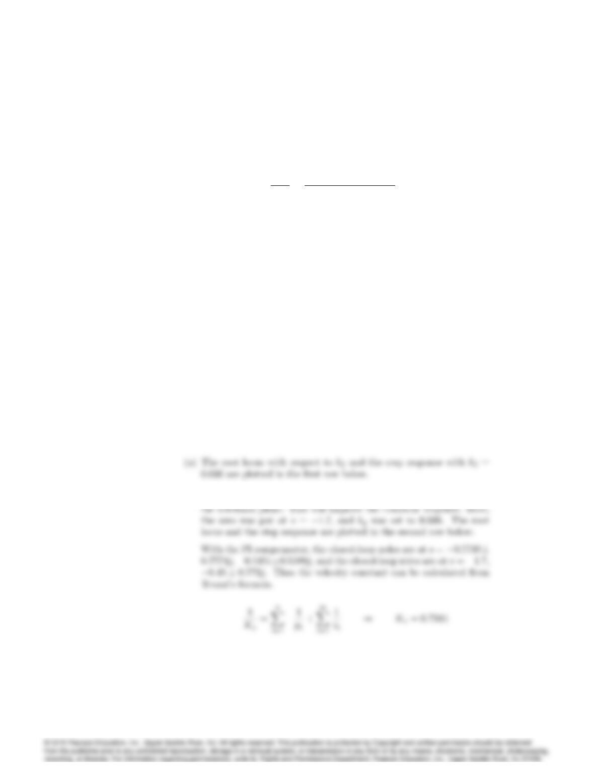
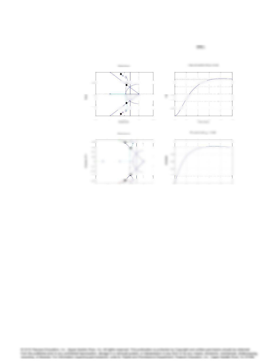
(b) Using rltool, we can choose the location of zeroto pull the locus to

-1

–0.5

1

0

0.4

0.8

1.2

-2 –1.5 -1 –0.5 0

–0.6

Real Axis

0 2 4 6 8 10

0.2

Time (sec )

Solution for Problem 5.37

5062 CHAPTER 5. THE ROOT-LOCUS DESIGN METHOD

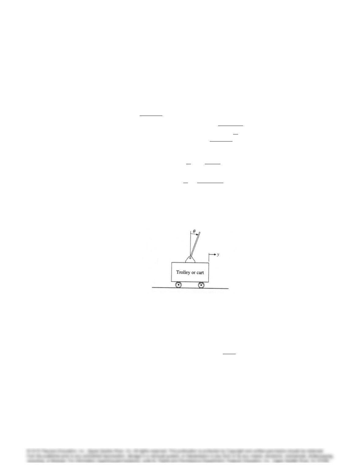
38. The normalized, scaled equations of a cart as drawn in Fig. 5.59 of mass

mcholding an inverted uniform pendulum of mass mpand length `with

no friction are •

=v

•y+ =v(5.88)

where =3mp

4(mc+mp)is a mass ratio bounded by 0<  < 0:75. Time is

measured in terms of =!otwhere !2

o=3g(mc+mp)

`(4mc+mp):The cart motion, y;

is measured in units of pendulum length as y=3x

4`and the input is force

normalized by the system weight, v=u

g(mc+mp):These equations can be

used to compute the transfer functions



V=1

s21(5.89)

Y

V=s21 + 

s2(s21) (5.90)

In this problem you are to design a control for the system by first closing

a loop around the pendulum, Eq.(5.89) and then, with this loop closed,

closing a second loop around the cart plus pendulum, Eq.(5.90). For this

problem, let the mass ratio be mc= 5mp:

Figure 5.59: Figure of cart-pendulum for Problem 5.38

(a) Draw a block diagram for the system with Vinput and both Yand

as outputs.

(b) Design a lead compensation Dc(s) = Ks+z

s+pfor the loop to cancel

the pole at s=1and place the two remaining poles at 4j4:The

new control is U(s), where the force is V(s) = U(s) + Dc(s)(s):

Draw the root locus of the angle loop.

(c) Compute the transfer function of the new plant from Uto Ywith

Dc(s)in place.

5063

(d) Design a controller Dc(s)for the cart position with the pendulum

loop closed. Draw the root locus with respect to the gain of Dc(s)

(e) Use Matlab to plot the control, cart position, and pendulum position

for a unit step change in cart position.

Solution:

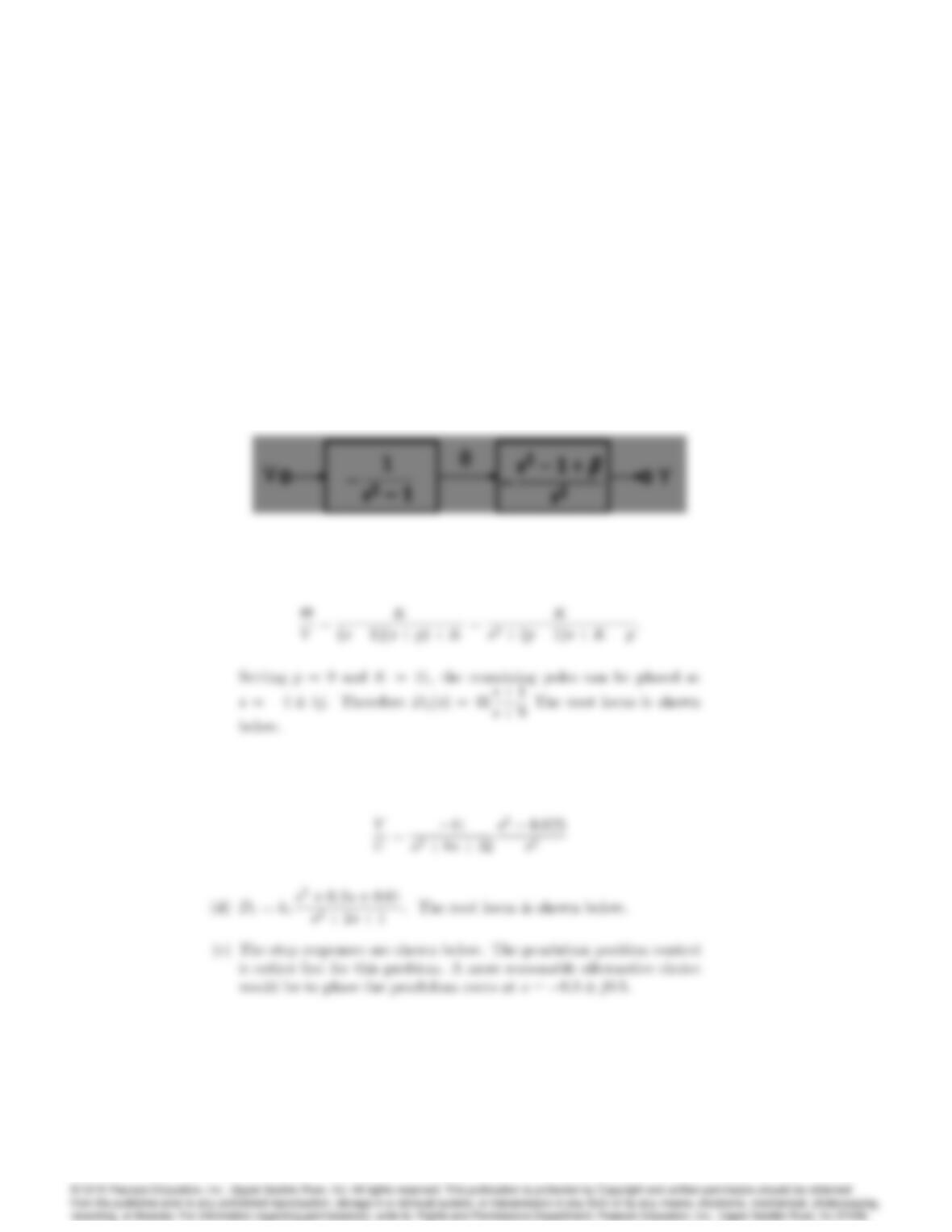
(a)

(b) To cancel the pole at s=1, we set z= 1. Then the closed loop

transfer function for the loop becomes

(c) Since mc= 5mp,= 0:125. Therefore the transfer function from U

to Ywith Dc(s)is

5064 CHAPTER 5. THE ROOT-LOCUS DESIGN METHOD

Inner pendulum loop

Real Axis

–10 -5 0

-2

4

Outer cart loop

Real Axis

-8 -6 -4 -2 0 2 4

-2

4

Final design

Time (sec)

050 100 150

–0.5

0

1.5

Alternative design

0

0.5

1.5

Alternative design

0.6

0.8

Root loci and step responses for Problem 5.38

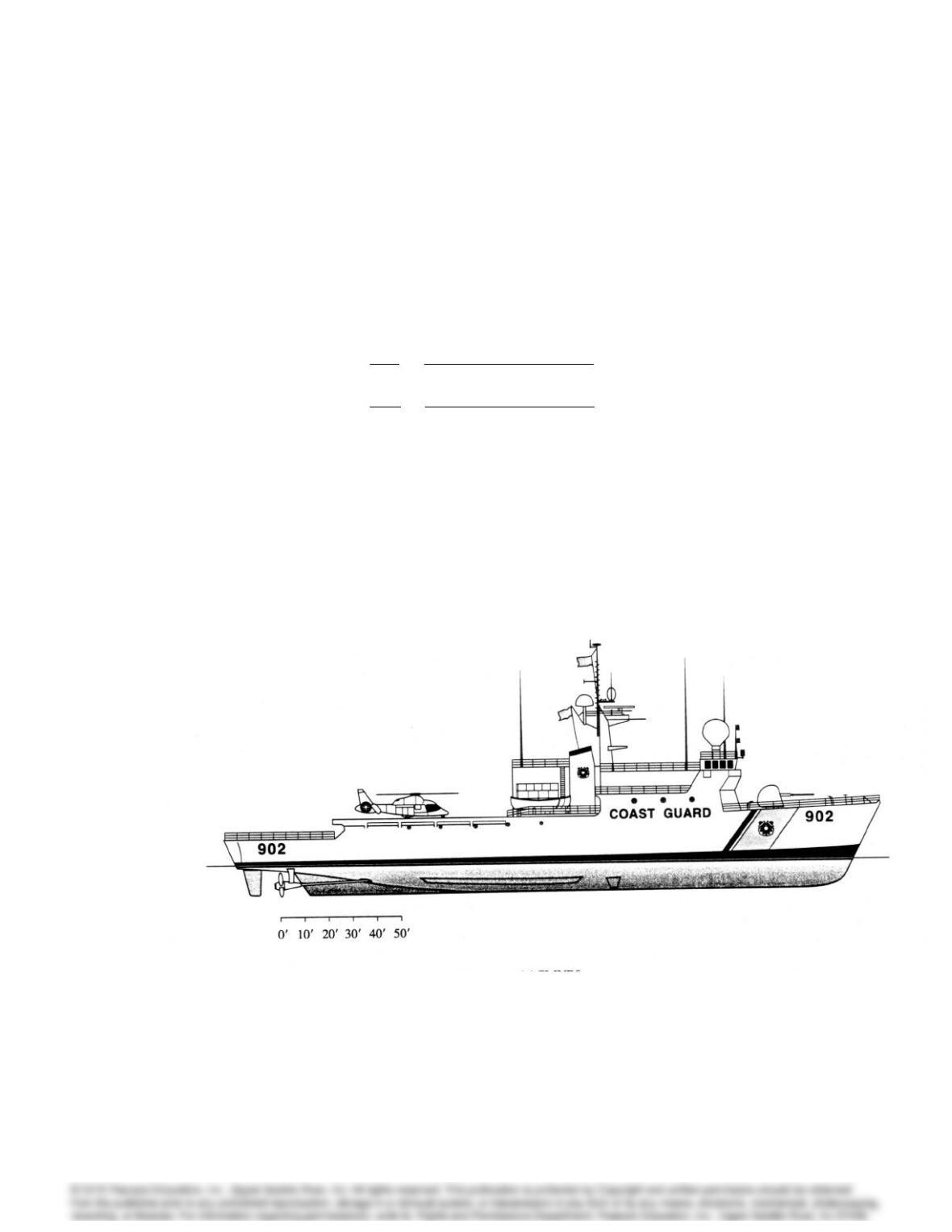
5065

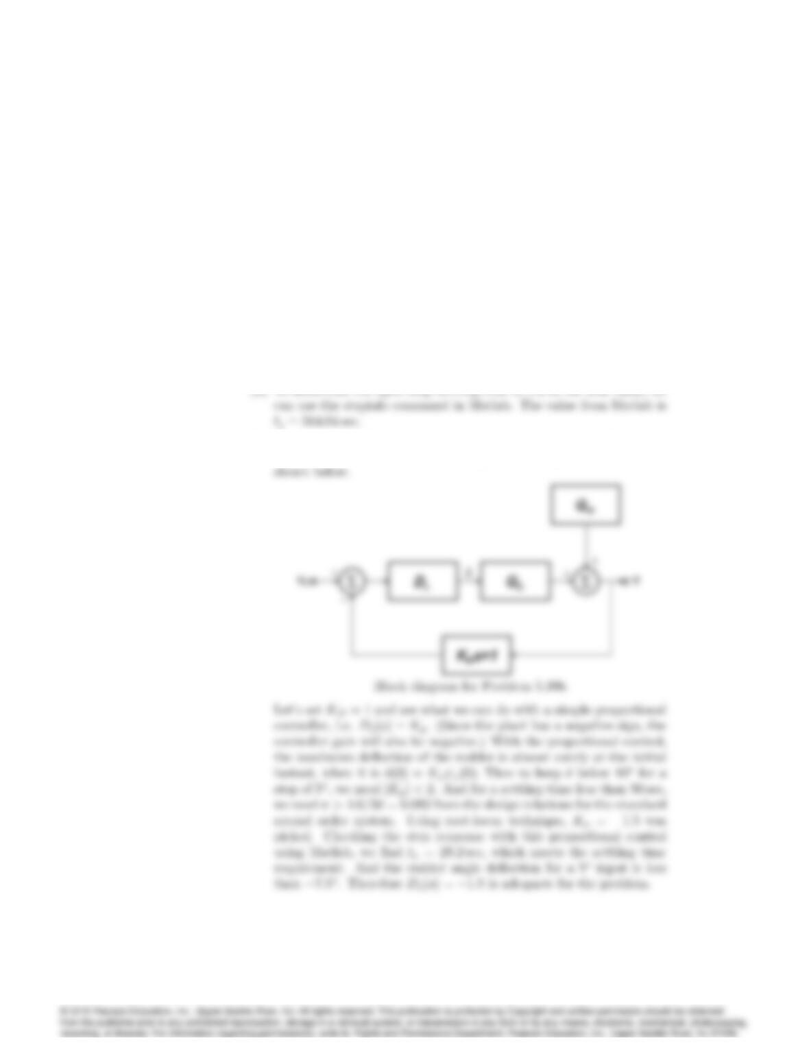
39. Consider the 270-ft U.S. Coast Guard cutter Tampa (902) shown in Fig. 5.60.

Parameter identification based on sea-trials data (Trankle, 1987) was used

to estimate the hydrodynamic coe¢cients in the equations of motion. The

result is that the response of the heading angle of the ship to rudder

angle and wind changes wcan be described by the second-order transfer

functions

G(s) = (s)

(s)=0:0184(s+ 0:0068)

s(s+ 0:2647)(s+ 0:0063);

Gw(s) = (s)

w(s)=0:0000064

s(s+ 0:2647)(s+ 0:0063);

where

=heading angle, rad

r=reference heading angle;rad:

r= yaw rate;rad=sec;

= rudder angle;rad;

w= wind speed;m=sec:

Figure 5.60: USCG cutter Tampa (902)

5066 CHAPTER 5. THE ROOT-LOCUS DESIGN METHOD

(a) Determine the open-loop settling time of rfor a step change in .

(b) In order to regulate the heading angle , design a compensator that

uses and the measurement provided by a yaw-rate gyroscope (that

is, by _

=r). The settling time of to a step change in ris specified

to be less than 50 sec, and, for a 5change in heading the maximum

allowable rudder angle de‡ection is specified to be less than 10.

(c) Check the response of the closed-loop system you designed in part (b)

to a wind gust disturbance of 10 m= sec (Model the disturbance as

a step input.) If the steady-state value of the heading due to this

wind gust is more than 0:5, modify your design so that it meets this

specification as well.

Solution:

(a) To determine the open-loop settling time to 1% of the final value, we

(b) The rate feedback from a yaw-rate gyroscope is giving us a derivative

control for free. Thus the block diagram of the system will look like

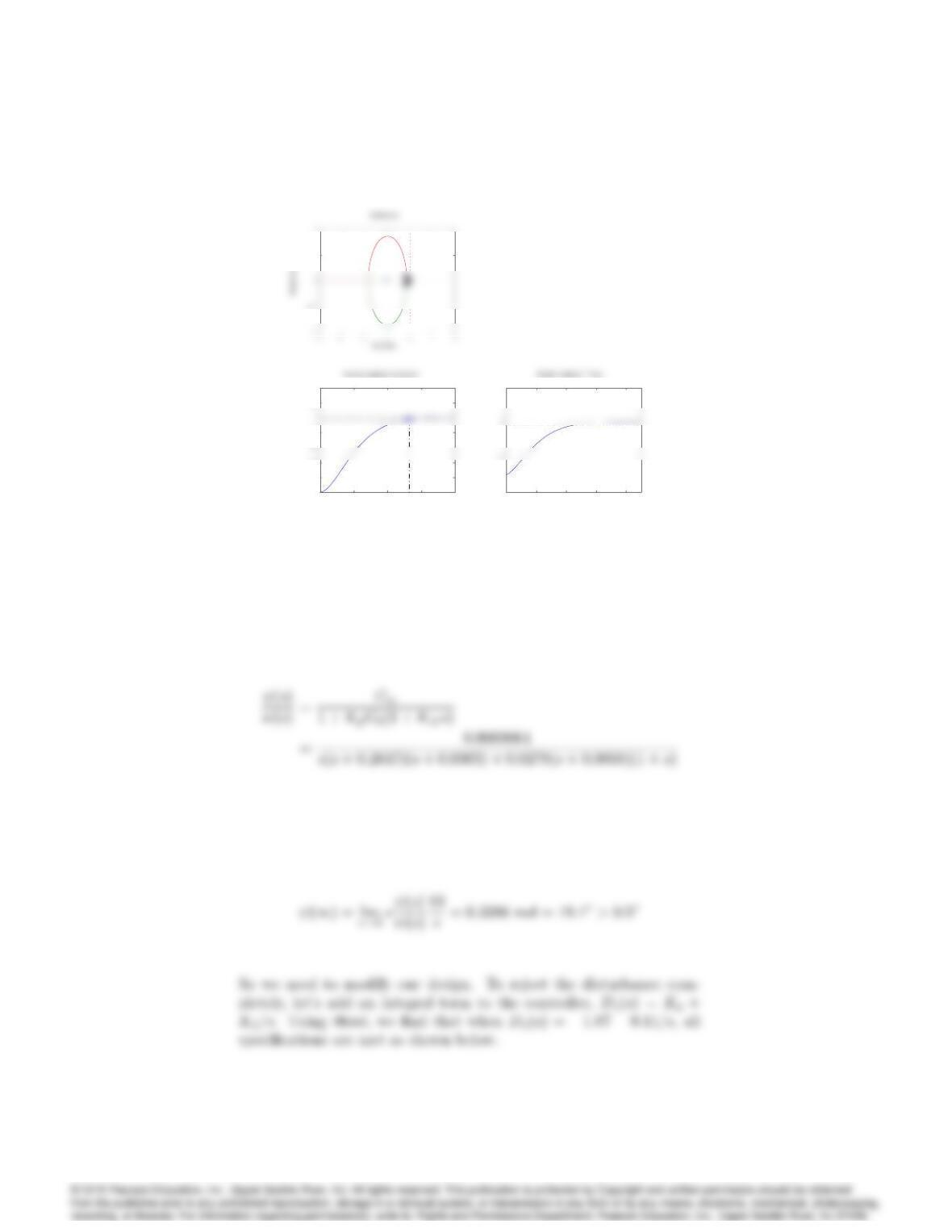
5067

0.5

010 20 30 40

0

0.2

0.4

0.8

1.2

1.4

Time (sec)

ψ

010 20 30 40

-10

5

Time (sec)

δ

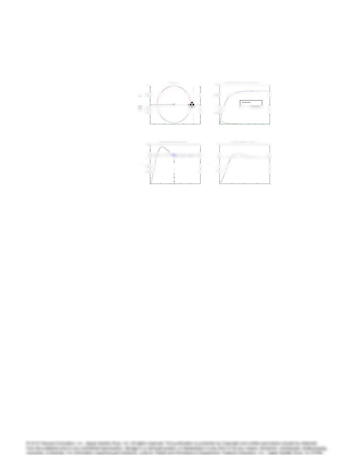
Root locus and Step response for Problem 5.39b

(c) With the compensator from part (b), the closed-loop transfer func-

tion from wto is

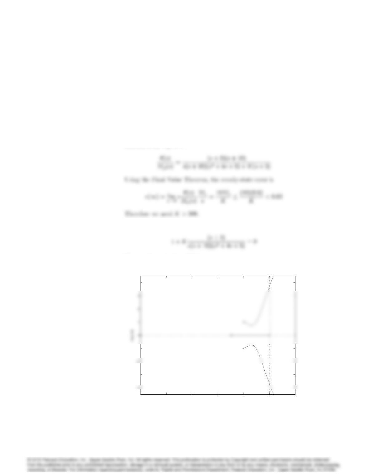
Using the Final Value Theorem, the steady-state value of the heading

angle due to a disturbance of 10m= sec is

5068 CHAPTER 5. THE ROOT-LOCUS DESIGN METHOD

-2 – 1 .5 -1 – 0.5 0

– 0 .8

– 0 .6

0.2

0.8

Root Locus

Real Ax is

020 40 60 80 100

0

0.2

0.8

1.2

Heading angle to a step input

Time (sec)

ψ

020 40 60 80

-10

Rudder angle to 5 o input

Time (sec)

δ

0200 400 600 800 1000 1200 1400

0

0.05

Heading angle to 10 m/s disturbance

Time (sec)

ψ

P control

Root locus and Step response for Problem 5.39c

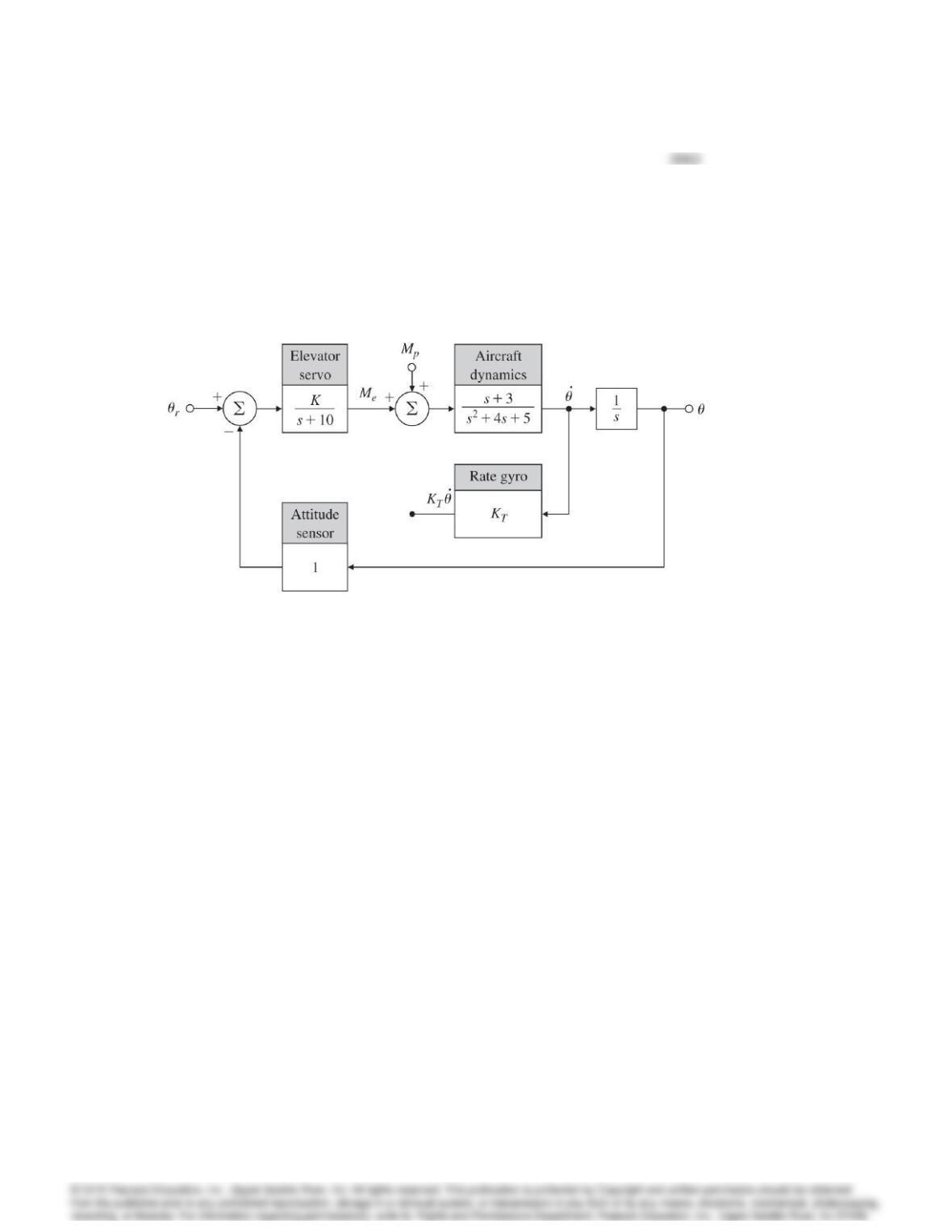
40. Golden Nugget Airlines has opened a free bar in the tail of their airplanes

in an attempt to lure customers. In order to automatically adjust for the

sudden weight shift due to passengers rushing to the bar when it first

opens, the airline is mechanizing a pitch-attitude auto pilot. Figure 5.61

shows the block diagram of the proposed arrangement. We will model the

passenger moment as a step disturbance Mp(s) = M0=s, with a maximum

expected value for M0of 0.6.

Figure 5.61: Golden Nugget Airlines Autopilot

(a) What value of Kis required to keep the steady-state error in to

less than 0.02 rad(

=1)? (Assume the system is stable.)

(b) Draw a root locus with respect to K.

(c) Based on your root locus, what is the value of Kwhen the system

becomes unstable?

(d) Suppose the value of Krequired for acceptable steady-state behavior

is 600. Show that this value yields an unstable system with roots at

s=2:9;13:5;+1:26:6j:

(e) You are given a black box with rate gyro written on the side and told

that when installed, it provides a perfect measure of _

, with output

KT_

. Assume K= 600 as in part (d) and draw a block diagram

indicating how you would incorporate the rate gyro into the auto

pilot. (Include transfer functions in boxes.)

(f) For the rate gyro in part (e), sketch a root locus with respect to KT.

(g) What is the maximum damping factor of the complex roots obtain-

able with the configuration in part (e)?

(h) What is the value of KTfor part (g)?

5070 CHAPTER 5. THE ROOT-LOCUS DESIGN METHOD

(i) Suppose you are not satisfied with the steady-state errors and damp-

ing ratio of the system with a rate gyro in parts (e) through (h).

Discuss the advantages and disadvantages of adding an integral term

and extra lead networks in the control law. Support your comments

using Matlab or with rough root-locus sketches.

Solution:

(a) Since any error is due to the disturbance Mp, we define the transfer

function from Mpto :

(b) The characteristic equation of the system in Evans form is

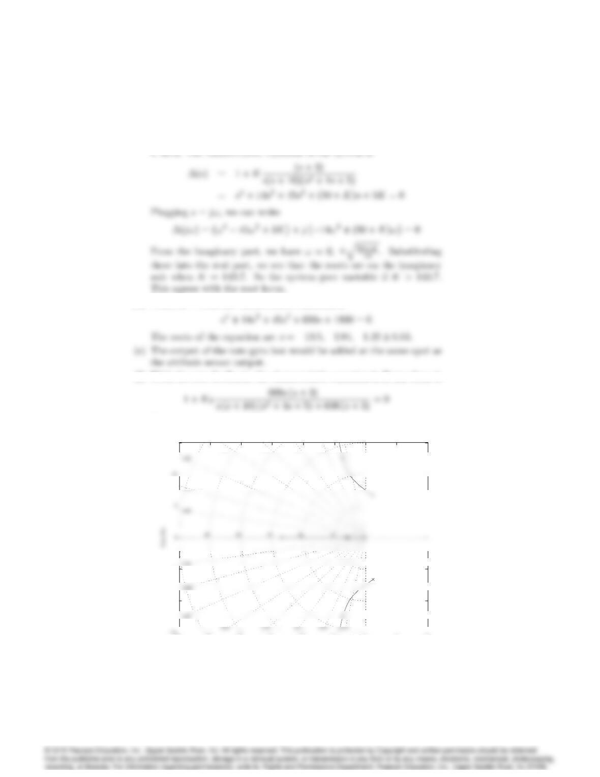
The root locus is plotted below.

Root locus for problem 5. 41

Real Axis

–10 -8 -6 -4 -2 0 2

-3

-1

4

5071

(c) To find the stability boundary, we can do the Routh test or solve the

characteristic equation for the j! crossings. Here, the latter method

is used. The characteristic equation of the system is

(d) When K= 600, the characteristic equation is

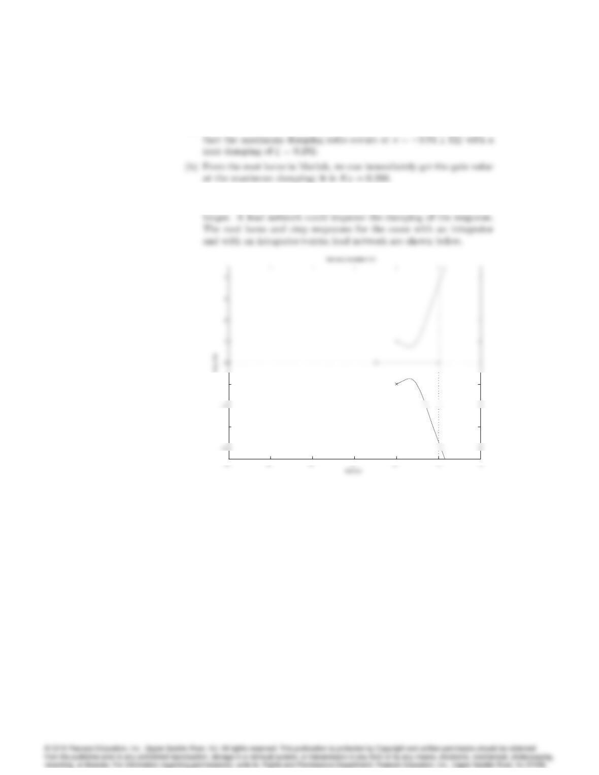
(f) With the rate feedback, the characteristic equation in Evans form is

The root locus is shown below.

Root Locus

Real Axis

-30 –25 -20 -15 –10 -5 0 5 10

-10

-5

15

0. 965

0. 84 0. 74 0.6 0. 42 0. 22

Root locus for Problem 5.40f

5072 CHAPTER 5. THE ROOT-LOCUS DESIGN METHOD

(g) From the root locus in Matlab, we can draw a point around and find

(i) Integral (PI) control would reduce the steady-state error to the mo-

ment to zero but would make the damping less and the settling time

Imag Axis

-3

-1

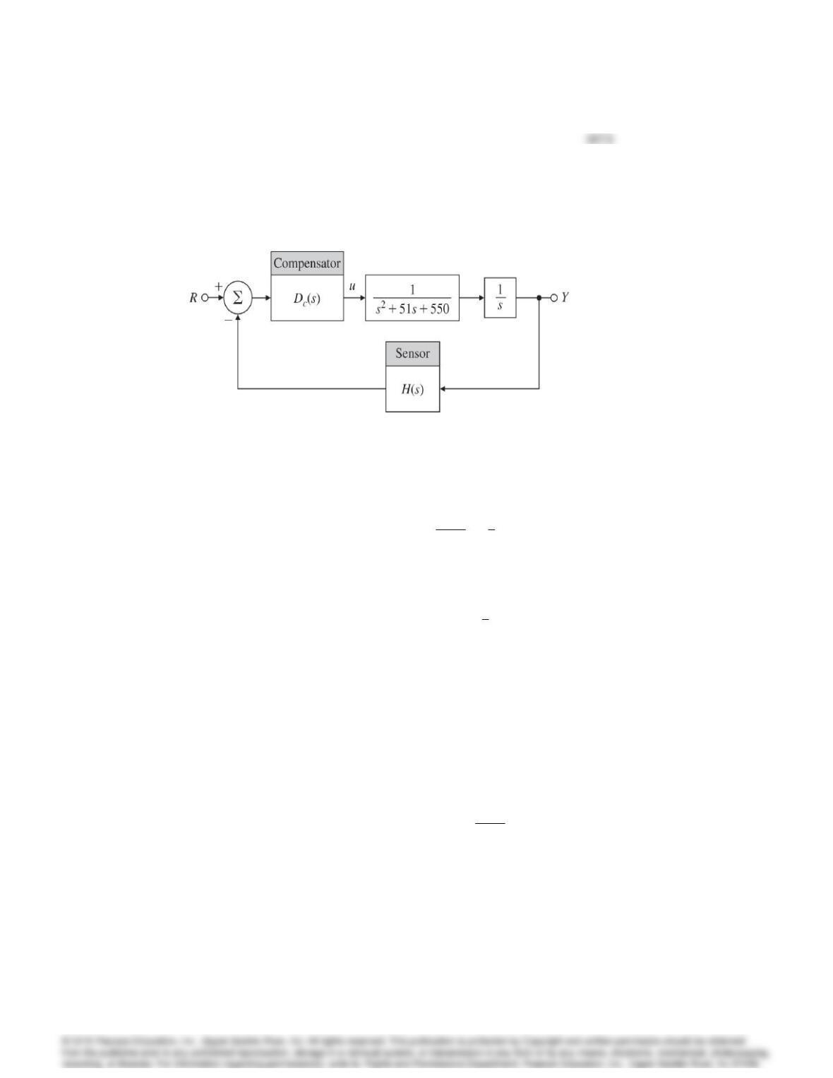
41. Consider the instrument servomechanism with the parameters given in

Fig. 5.62. For each of the following cases, draw a root locus with respect

to the parameter K, and indicate the location of the roots corresponding

to your final design.

Figure 5.62: Control system for Problem 5.41

(a) Lead network : Let

H(s) = 1; Dc(s) = Ks+z

s+p;p

z= 6:

Select zand Kso that the roots nearest the origin (the dominant

roots) yield

0:4; 7; Kv162

3sec1:

(b) Output-velocity (tachometer) feedback : Let

H(s) = 1 + KTsand Dc(s) = K:

Select KTand Kso that the dominant roots are in the same location

as those of part (a). Compute Kv. If you can, give a physical rea-

son explaining the reduction in Kvwhen output derivative feedback

is used.

(c) Lag network : Let

H(s) = 1 and D(s) = Ks+ 1

s+p:

Using proportional control, is it possible to obtain a Kv= 12 at

= 0:4? Select Kand pso that the dominant roots correspond to the

proportional-control case but with Kv= 100 rather than Kv= 12.

5074 CHAPTER 5. THE ROOT-LOCUS DESIGN METHOD

Solution:

(a) Setting p= 6z, the velocity constant is

-45 -40 –35 -30 –25 -20 -15 -10 -5 0 5

-20

Root locus with respect to z

Rea l Ax is

Root locus for Problem 5.41(a)

(b) With H(s) = 1 + KTsand Dc(s) = K, the closed-loop transfer