
5000
Solutions Manual: Chapter 5
7th Edition
Feedback Control of Dynamic
Systems
Gene F. Franklin
J. David Powell
Abbas Emami-Naeini .
Assisted by:
H.K. Aghajan
H. Al-Rahmani
P. Coulot
P. Dankoski
S. Everett
R. Fuller
T. Iwata
V. Jones
F. Safai
L. Kobayashi
H-T. Lee
E. Thuriyasena
M. Matsuoka
J.K. Lee

Chapter 5
The Root–Locus Design
Method
Problems and solutions for Section 5.1
1. Set up the listed characteristic equations in the form suited to Evans’s
root-locus method. Give L(s); a(s);and b(s)and the parameter Kin
terms of the original parameters in each case. Be sure to select Kso that
a(s)and b(s)are monic in each case and the degree of b(s)is not greater
than that of a(s).
(a) s+ (1=) = 0 versus parameter
(b) s2+cs +c+ 1 = 0 versus parameter c
(c) (s+c)3+A(T s + 1) = 0
i. versus parameter A,
ii. versus parameter T,
iii. versus the parameter c, if possible. Say why you can or can not.
Can a plot of the roots be drawn versus cfor given constant
values of Aand Tby any means at all?
(d) 1+kp+kI
s+kDs
s + 1G(s) = 0:Assume that G(s) = Ac(s)
d(s), where
c(s)and d(s)are monic polynomials with the degree of d(s)greater
than that of c(s). (Note: The first printing of the 7th edition
had an error in the equation above where the kI
sterm above was
incorrectly stated to be kI(s):)
i. versus kp
ii. versus kI
iii. versus kD
5001
5002 CHAPTER 5. THE ROOT-LOCUS DESIGN METHOD
iv. versus
Solution:
(c) i. K=AT ;
(d) i. K=kpA;
5003
Problems and solutions for Section 5.2
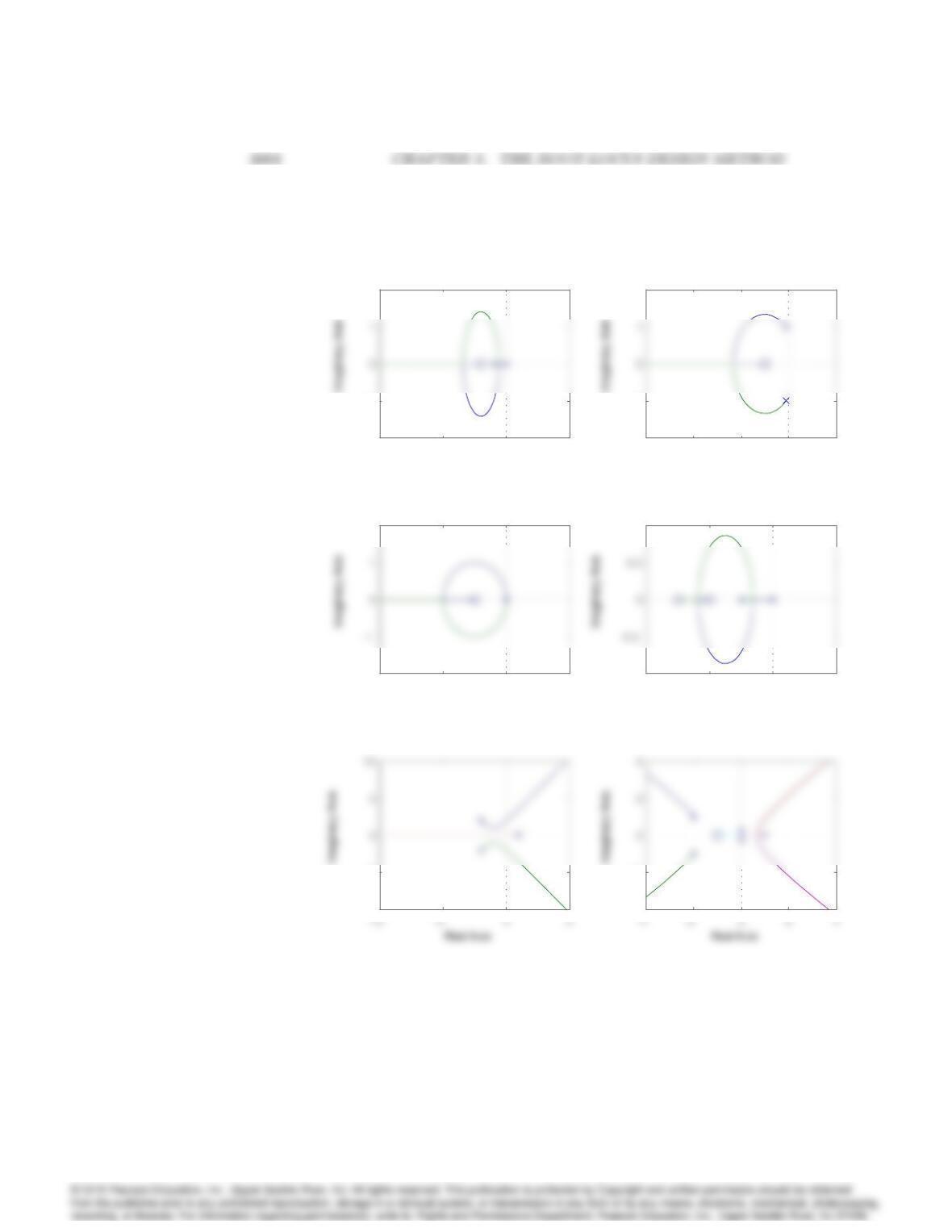
2. Roughly sketch the root loci for the pole-zero maps as shown in Fig. 5.44
without the aid of a computer. Show your estimates of the center and
angles of the asymptotes, a rough evaluation of arrival and departure
angles for complex poles and zeros, and the loci for positive values of the
parameter K. Each pole-zero map is from a characteristic equation of the
form
1 + Kb(s)
a(s)= 0;
where the roots of the numerator b(s)are shown as small circles oand the
roots of the denominator a(s)are shown as 0son the s-plane. Note that
in Fig. 5.44(c) there are two poles at the origin.
Solution:
We had to make up some numbers to do it on Matlab, so the results
partly depend on what was dreamed up, but the idea here is just get the
basic rules right.
(a) a(s) = s2+s;b(s) = s+ 2
(d) a(s) = s2+s;b(s) = s2+ 5s+ 6
–10 -5 0 5
-2
-1
2
Root loci for Problem 5.2
Real Axis
-6 -4 -2 0 2
-2
-1
2
Real Axis
-4 -2 0 2
-2
2
Real Axis
-4 -2 0 2
-1
1
Real Axis
–10
-5
-4
-2
3. For the characteristic equation
1 + K
s2(s+ 1)(s+ 5) = 0;
(a) Draw the real-axis segments of the corresponding root locus.
(b) Sketch the asymptotes of the locus for K! 1.
(c) Sketch the locus.
(d) Verify your sketch with a Matlab plot.
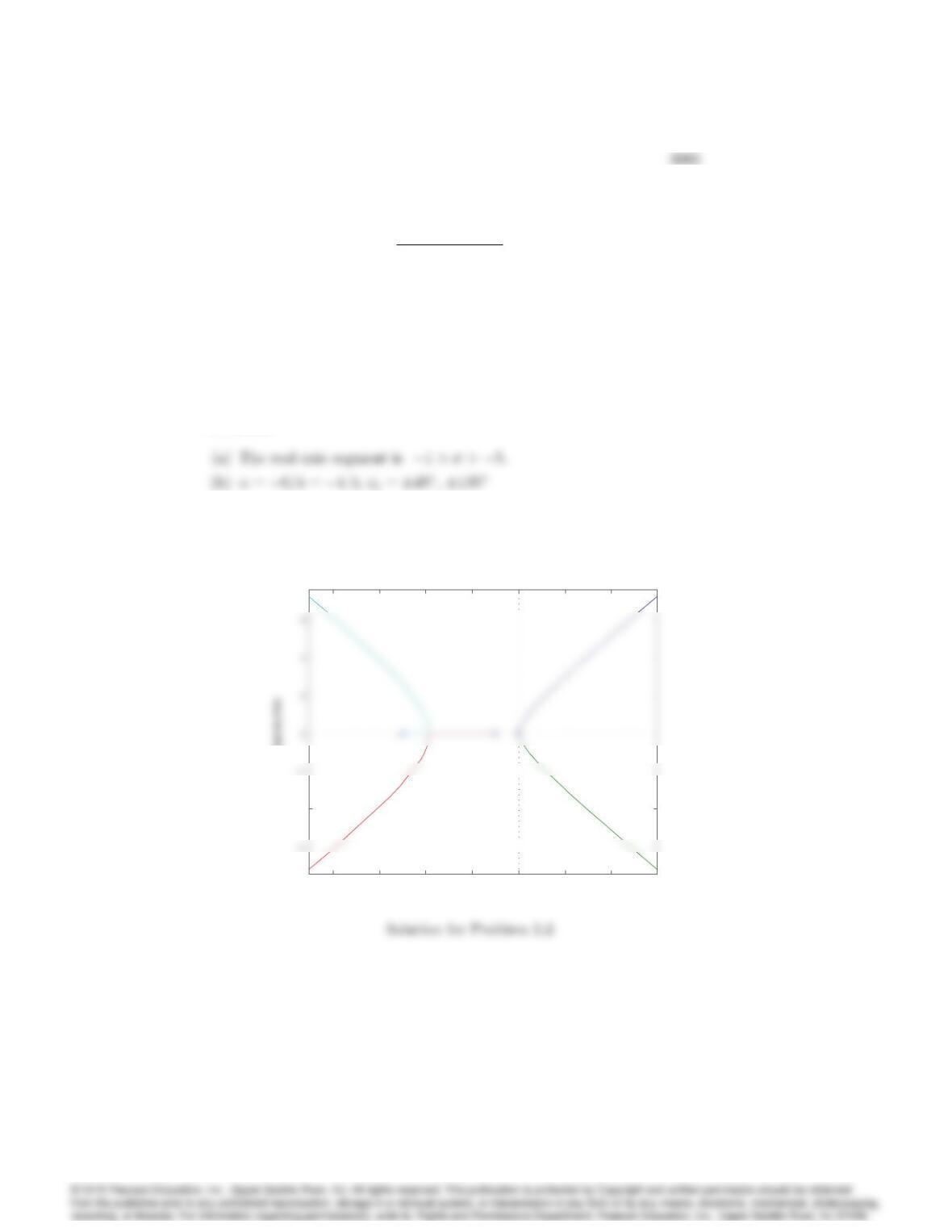
Solution:
(c) The plot is shown below.
-8 -6 -4 -2 0 2 4
-4
Root Locus
Real Axis
Imaginary Axis

5006 CHAPTER 5. THE ROOT-LOCUS DESIGN METHOD
4. Real poles and zeros. Sketch the root locus with respect to Kfor the
equation 1+KL(s) = 0 and the listed choices for L(s). Be sure to give the
asymptotes and the arrival and departure angles at any complex zero or
pole. After completing each hand sketch, verify your results using Matlab.
Turn in your hand sketches and the Matlab results on the same scales.
(a) L(s) = 2
s(s+ 1)(s+ 5)(s+ 10)
(b) L(s) = (s+ 3)
s(s+ 1)(s+ 5)(s+ 10)
(c) L(s) = (s+ 2)(s+ 4)
s(s+ 1)(s+ 5)(s+ 10)
(d) L(s) = (s+ 2)(s+ 6)
s(s+ 1)(s+ 5)(s+ 10)
Solution:
All the root locus plots are displayed at the end of the solution set for this
problem.
5007
-15 –10 -5 0 5
-15
Real Axis
-15 –10 -5 0 5
-15
Real Axis
-15 –10 -5 0 5
-10
c
Real Axis
-15 –10 -5 0 5
-10
d
Real Axis
Root loci for Problem 5.4
5. Complex poles and zeros. Sketch the root locus with respect to Kfor the
equation 1+KL(s) = 0 and the listed choices for L(s). Be sure to give the
asymptotes and the arrival and departure angles at any complex zero or
pole. After completing each hand sketch, verify your results using Matlab.
Turn in your hand sketches and the Matlab results on the same scales.
(a) L(s) = 1
s2+ 3s+ 10
(b) L(s) = 1
s(s2+ 3s+ 10)
(c) L(s) = (s2+ 2s+ 8)
s(s2+ 2s+ 10)
(d) L(s) = (s2+ 2s+ 12)
s(s2+ 2s+ 10)
(e) L(s) = (s2+ 1)
s(s2+ 4)
(f) L(s) = (s2+ 4)
s(s2+ 1)
Solution:
All the root locus plots are displayed at the end of the solution set for this
problem.
5009
-3 -2 -1 0 1
–10
a
Real Axis
Imaginary Axis
–20 –10 010
–10
b
Real Axis
Imaginary Axis
-3 -2 -1 0 1
-4
c
Real Axis
-3 -2 -1 0 1
-4
d
Real Axis
-2 -1 0 1
-4
e
Real Axis
–1.5 -1 –0.5 00.5
-4
f
Real Axis
Root loci for Problem 5.5
6. Multiple poles at the origin. Sketch the root locus with respect to Kfor
the equation 1 + KL(s) = 0 and the listed choices for L(s). Be sure to
give the asymptotes and the arrival and departure angles at any complex
zero or pole. After completing each hand sketch, verify your results using
Matlab. Turn in your hand sketches and the Matlab results on the same
scales.
(a) L(s) = 1
s2(s+ 8)
(b) L(s) = 1
s3(s+ 8)
(c) L(s) = 1
s4(s+ 8)
(d) L(s) = (s+ 3)
s2(s+ 8)
(e) L(s) = (s+ 3)
s3(s+ 4)
(f) L(s) = (s+ 1)2
s3(s+ 4)
(g) L(s) = (s+ 1)2
s3(s+ 10)2
Solution:
All the root locus plots are displayed at the end of the solution set for this
problem.
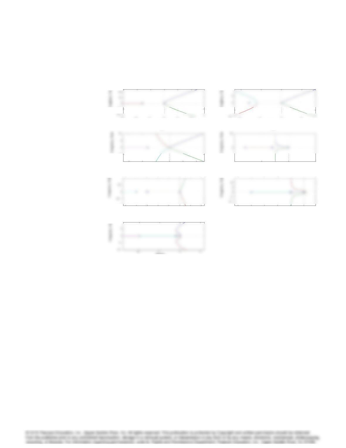
5011
–15 – 10 -5 0 5 10
–10
a
Real Axis
I m aginary Axis
–10 -5 0 5
-5
b
Real Axis
I m aginary Axis
–15 – 10 -5 0 5 10
-5
c
Real Axis
–10 -5 0 5
–50
d
Real Axis
-5 -4 -3 -2 -1 0 1 2
-1
e
Real Axis
-5 -4 -3 -2 -1 0
f
Real Axis
g
Real Axis
Solution for Problem 5.6

5012 CHAPTER 5. THE ROOT-LOCUS DESIGN METHOD
7. Mixed real and complex poles. Sketch the root locus with respect to Kfor
the equation 1 + KL(s) = 0 and the listed choices for L(s). Be sure to
give the asymptotes and the arrival and departure angles at any complex
zero or pole. After completing each hand sketch, verify your results using
Matlab. Turn in your hand sketches and the Matlab results on the same
scales.
(a) L(s) = (s+ 3)
s(s+ 10)(s2+ 2s+ 2)
(b) L(s) = (s+ 3)
s2(s+ 10)(s2+ 6s+ 25)
(c) L(s) = (s+ 3)2
s2(s+ 10)(s2+ 6s+ 25)
(d) L(s) = (s+ 3)(s2+ 4s+ 68)
s2(s+ 10)(s2+ 4s+ 85)
(e) L(s) = [(s+ 1)2+ 1]
s2(s+ 2)(s+ 3)
Solution:
All the plots are attached at the end of the solution set.
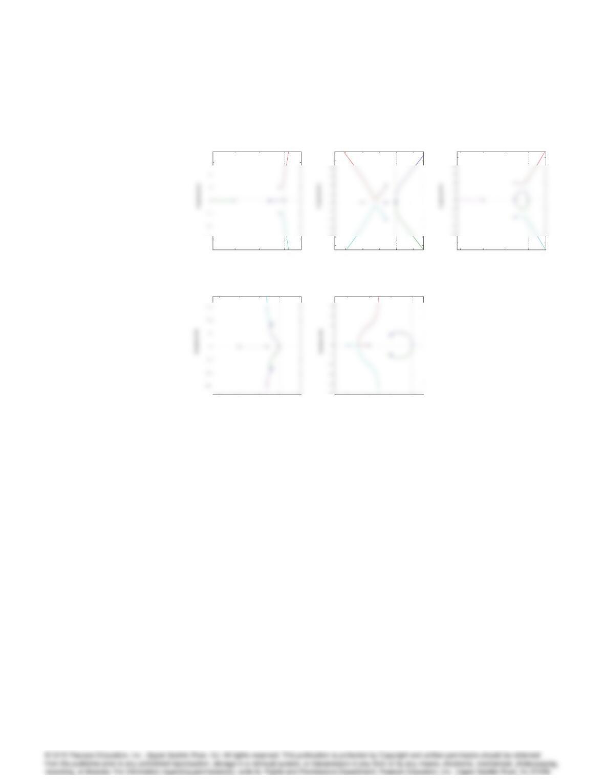
5013
-10 -5 0
-3
3
a
Real Axis
-15 –10 -5 0 5
-10
-8
10
b
Real Axis
-15 –10 -5 0
-10
10
c
Real Axis
-15 –10 -5 0 5
d
Real Axis
-3 -2 -1 0
-5
5
e
Real Axis
Solution for Problem 5.7
5014 CHAPTER 5. THE ROOT-LOCUS DESIGN METHOD
8. RHP and zeros. Sketch the root locus with respect to Kfor the equa-
tion 1 + KL(s) = 0 and the listed choices for L(s). Be sure to give the
asymptotes and the arrival and departure angles at any complex zero or
pole. After completing each hand sketch, verify your results using Matlab.
Turn in your hand sketches and the Matlab results on the same scales.
(a) L(s) = s+ 2
s+ 10
1
s21;the model for a case of magnetic levitation
with lead compensation.
(b) L(s) = s+ 2
s(s+ 10)
1
(s21);the magnetic levitation system with inte-
gral control and lead compensation.
(c) L(s) = s1
s2
(d) L(s) = s2+ 2s+ 1
s(s+ 20)2(s22s+ 2):What is the largest value that can
be obtained for the damping ratio of the stable complex roots on this
locus?
(e) L(s) = (s+ 2)
s(s1)(s+ 6)2;
(f) L(s) = 1
(s1)[(s+ 2)2+ 3]
Solution:

5015
-10 -5 0
-10
Real Axis
Imag Axis
-10 -5 0
-10
Real Axis
Imag Axis
-1 0 1 2
-1
Real Axis
Imag Axis
-15
Real Axis
t d
10
Real Axis
4
Real Axis
Solution for Problem 5.8
5016 CHAPTER 5. THE ROOT-LOCUS DESIGN METHOD
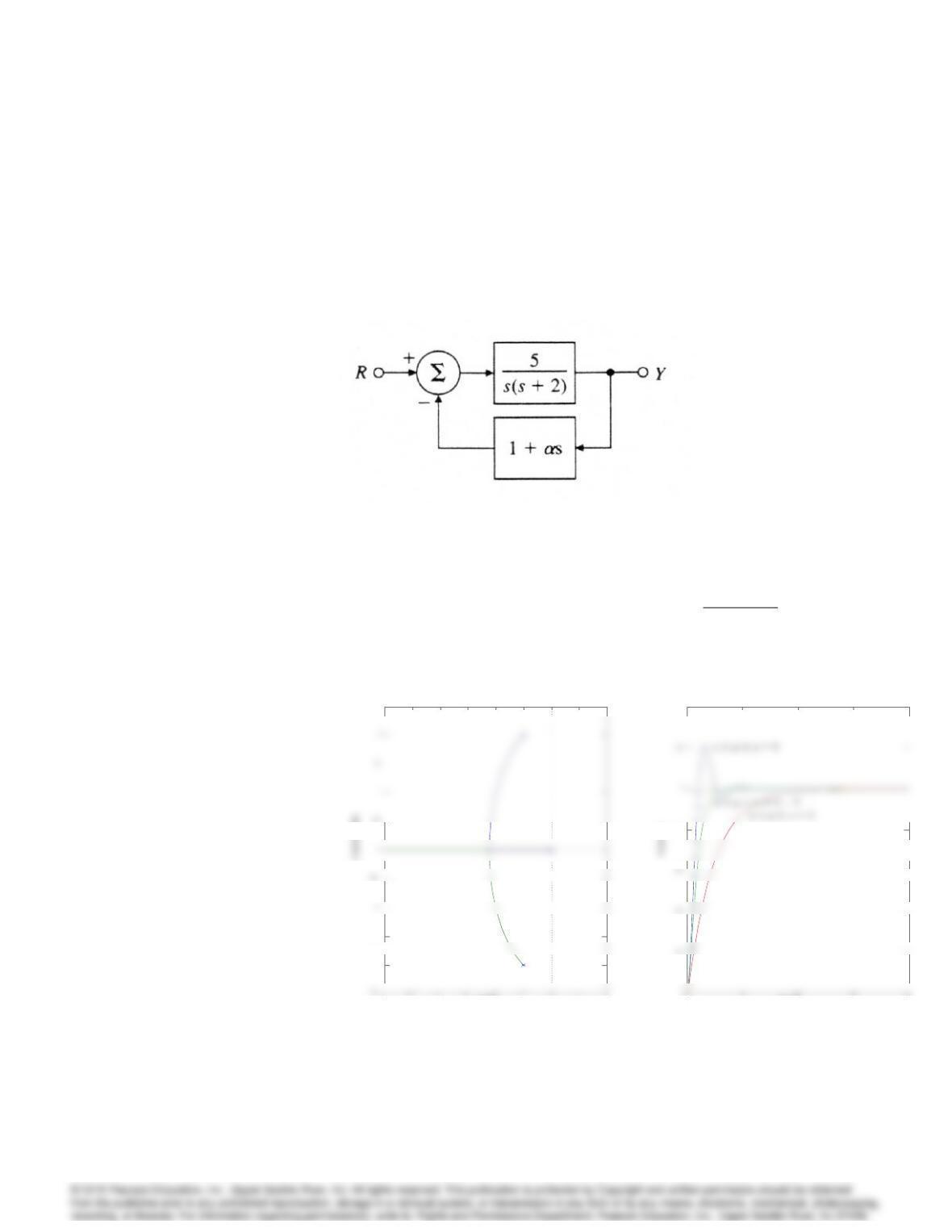
9. Put the characteristic equation of the system shown in Fig. 5.45 in root
locus form with respect to the parameter , and identify the corresponding
L(s); a(s);and b(s):Sketch the root locus with respect to the parameter
, estimate the closed-loop pole locations, and sketch the corresponding
step responses when = 0;0:5, and 2. Use Matlab to check the accuracy
of your approximate step responses.
Figure 5.45: Control system for Problem 5.9
Solution:
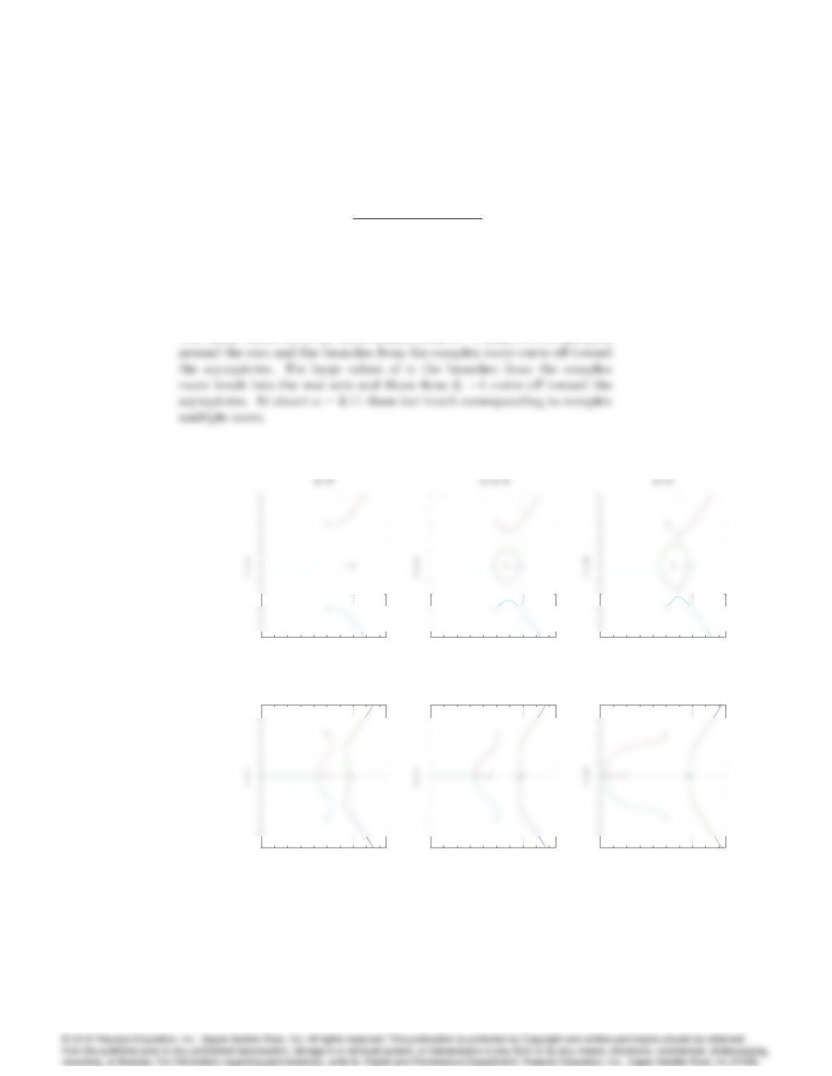
The characteristic equation is s2+2s+5+5s = 0 and L(s) = s
s2+ 2s+ 5:
the root locus and step responses are plotted below.
-6 -5 -4 -3 -2 -1 0 1 2
-2
-1.5
0.5
2.5
root l ocus
Real Axis
0 5 10 15 20
0.8
1.4
S t ep Res po ns e
Ti me (sec)
5017
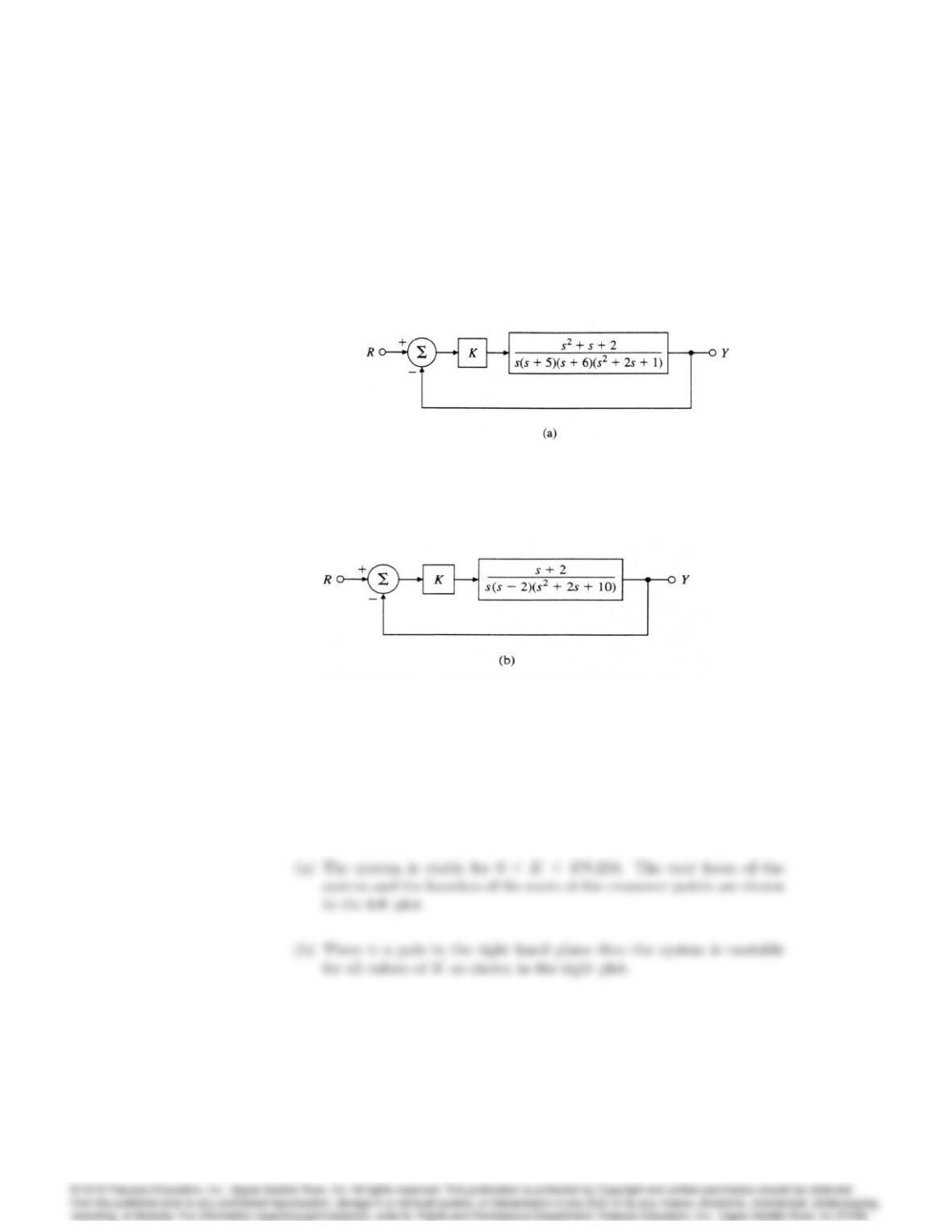
10. Use the Matlab function rltool to study the behavior of the root locus of
1 + KL(s)for
L(s) = (s+a)
s(s+ 1)(s2+ 8s+ 52)
as the parameter ais varied from 0to 10, paying particular attention to
the region between 2:5and 3:5. Verify that a multiple root occurs at a
complex value of sfor some value of ain this range.
Solution:
For small values of ; the locus branch from 0;1makes a circular path
–14 -12 –10 -8 -6 -4 -2 0 2 4
–10
-4
R eal Axis
–14 -12 –10 -8 -6 -4 -2 0 2 4
–10
-4
R eal Axis
–14 -12 –10 -8 -6 -4 -2 0 2 4
–10
-4
R eal Axis
–14 -12 –10 -8 -6 -4 -2 0 2 4
–10
10
a=3.5
R eal Axis
–14 -12 –10 -8 -6 -4 -2 0 2 4
–10
10
a=5
R eal Axis
–14 -12 –10 -8 -6 -4 -2 0 2 4
–10
10
a=10
R eal Axis
Solution for Problem 5.10
5018 CHAPTER 5. THE ROOT-LOCUS DESIGN METHOD
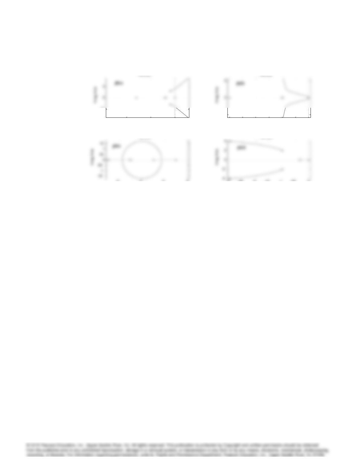
11. Use Routh’s criterion to find the range of the gain Kfor which the systems
in Fig. 5.46 are stable, and use the root locus to confirm your calculations.
Figure 5.46: Feedback systems for Problem 5.11
Solution:
5019
Root Lo c us
Real Axis
– 10 -5 0
-5
Root Lo c us
Real Axis
-3 –2.5 -2 –1.5 -1 –0.5 0
-5
Root Lo c us
Real Axis
-6 -4 -2 0
Root Lo c us
Real Axis
-3 –2.5 -2 –1.5 -1 –0.5 0
Solution for Problem 5.11