5075
(c) Using proportional control (Dc(s) = K), the velocity constant is
With Dc(s) = Ks+1
s+p, the velocity constant is
-40 -35 -30 -25 -20 -15 -10 -5 0 5 10
-20
-10
0
5
10
15
20
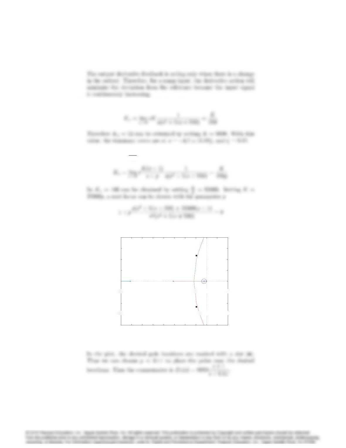
Root locus with respect to p
Real Ax is
Ima gin a r y Axis
Root locus for Problem 5.41(c)
5076 CHAPTER 5. THE ROOT-LOCUS DESIGN METHOD
Problems and solutions for Section 5.6
42. Plot the loci for the 0locus or negative Kfor each of the following:
(a) The examples given in Problem 5.3
(b) The examples given in Problem 5.4
(c) The examples given in Problem 5.5
(d) The examples given in Problem 5.6
(e) The examples given in Problem 5.7
(f) The examples given in Problem 5.8
Solution:
(a)
-15 -10 -5 0 5 10 15
-10
Real Axis
Problem 5.42(a)
5077
-15 –10 -5 0 5 10
6
8
10
plot a
Real Axis
-15 –10 -5 0 5 10
10
15
20
plot b
Real Axis
-20 -15 –10 -5 0 5
-1
–0.5
1
2
plot c
Real Axis
-10 -8 -6 -4 -2 0 2
-1
–0.5
0.5
1
plot d
Real Axis
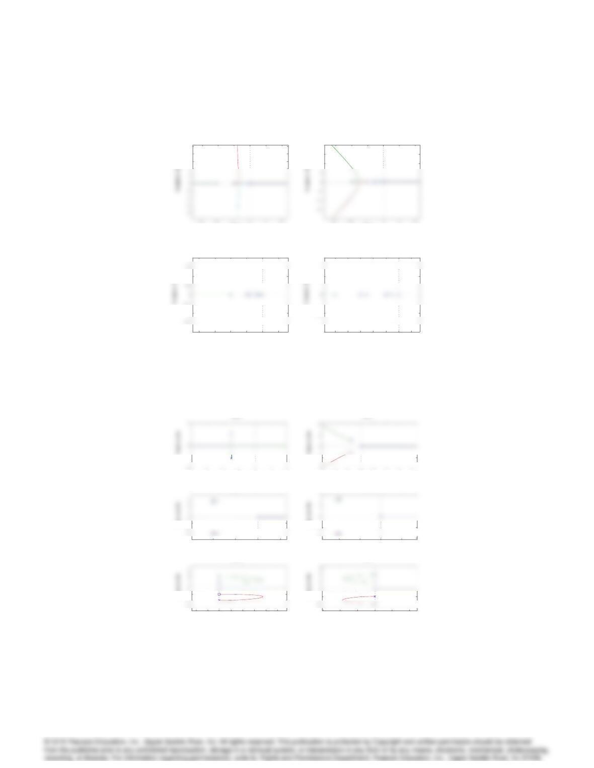
Problem 5.42(b)
-4 -3 -2 -1 0 1 2
plot a
Re al Ax is
-6 -4 -2 02468
-5
plot b
Re al Ax is
-1 – 0 .5 00.5
-1
plot c
Re al Ax is
Imagina ry Axis
-1 – 0 .5 00.5
-4
plot d
Re al Ax is
Imagina ry Axis
– 0 .4 – 0 .2 00 .2 0.4 0 .6 0.8 1
-1
plot e
Re al Ax is
Imagina ry Axis
– 0 .6 – 0 .4 – 0 .2 00.2 0.4
-3
-1
plot f
Re al Ax is
Imagina ry Axis
Problem 5.42(c)
5078 CHAPTER 5. THE ROOT-LOCUS DESIGN METHOD
–20 –10 010 20 30 40
–50
Real Axis
–20 –10 010
Real Axis
–20 –10 010
–20
plo t c
Real Axis
–15 –10 -5 0 5 10
-1
plo t d
Real Axis
–10 -5 0 5
–10
plo t e
Real Axis
–10 -5 0 5
– 0.5
plo t f
Real Axis
–20 –10 010
–20
g
Real Axis
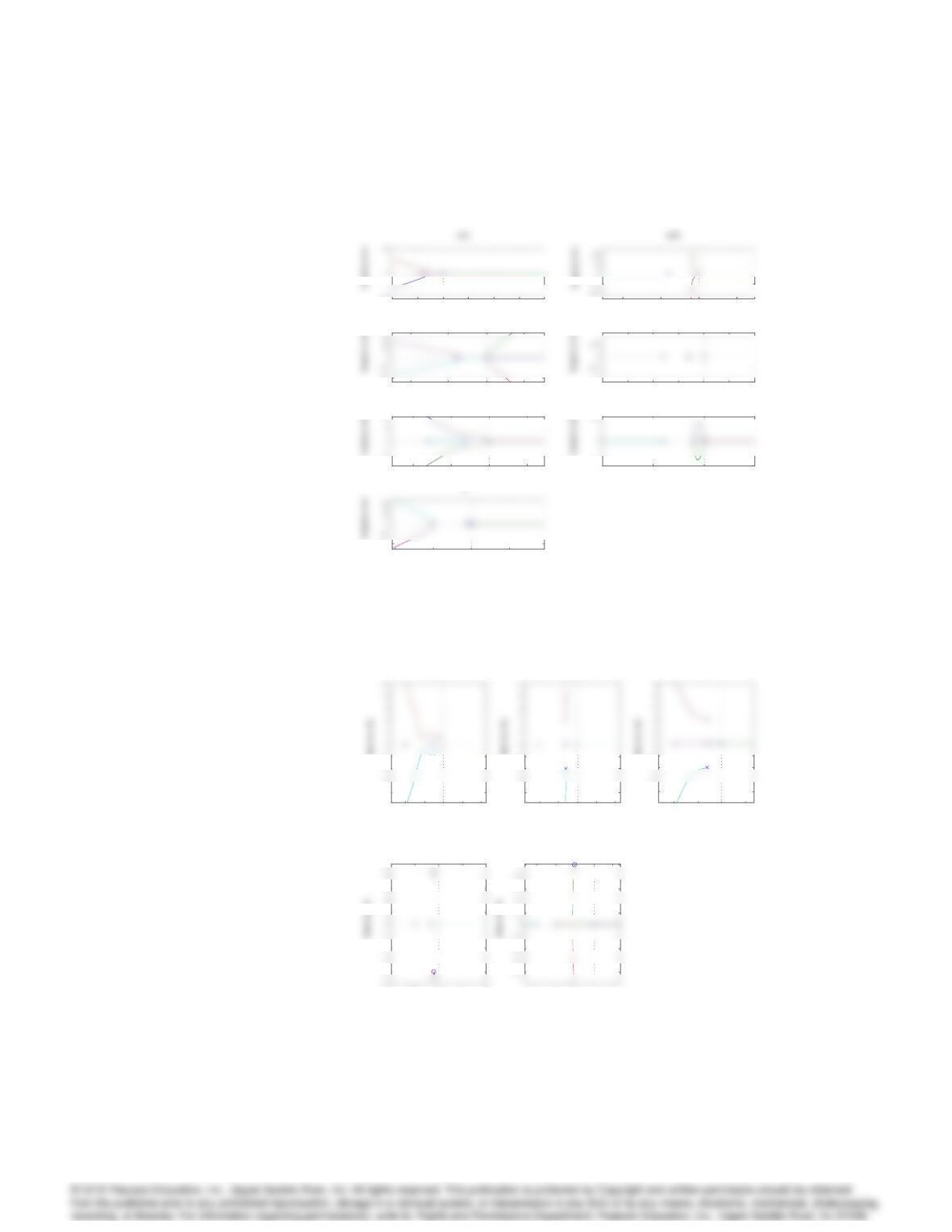
Problem 5.42(d)
-10 -5 0 5 10
-8
-6
-2
plot a
Real Axis
Imaginary Axis
-10 -5 0 5 10
-8
-6
-2
plot b
Real Axis
Imaginary Axis
-10 -5 0 5
-8
-2
plot c
Real Axis
Imaginary Axis
-20 –10 010 20
-4
6
plot d
Real Axis
-3 -2 -1 0 1
plot e
Real Axis
Problem 5.42(e)

5079
–15 –10 -5 0 5
-0.8
-0.4
0.4
0.6
plot a
Real A xis
–10 -5 0
-4
-2
-1
2
3
4
plot b
Real A xis
-2 0 2 4
-2
-1
-0.5
0.5
1
1.5
plot c
Real A xis
–30 –20 – 10 0
-8
-6
-2
plot d
Real A xis
Im aginar y Axis
–10 -5 0
-8
-6
-2
plot e
Real A xis
Im aginar y Axis
-5 0 5
-4
-3
-1
plot f
Real A xis
Im aginar y Axis
Problem 5.42(f)
43. Suppose you are given the plant
L(s) = 1
s2+ (1 + )s+ (1 + );
where is a system parameter that is subject to variations. Use both
positive and negative root-locus methods to determine what variations in
can be tolerated before instability occurs.
Solution:
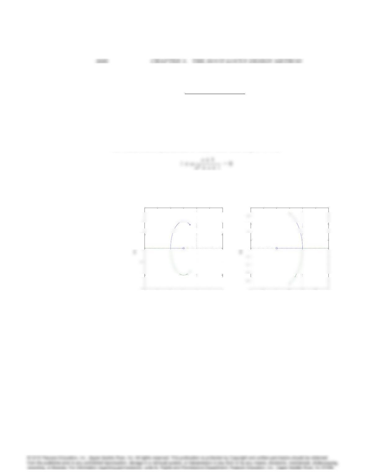
The characteristic polynomial in Evans form with respect to is
The positive and negative root locus are shown below.
-4 -3 -2 -1 0 1 2
-1
0.5
1.5
Positive root locus
Real Axis
-2 – 1 .5 -1 – 0 .5 00 .5 1
0.2
0.6
1
Negative root locus
Real Axis
Positive(left) and Negative(right) root locus for Problem 5.43
From the root locus, we see that the system is stable for all > 1.
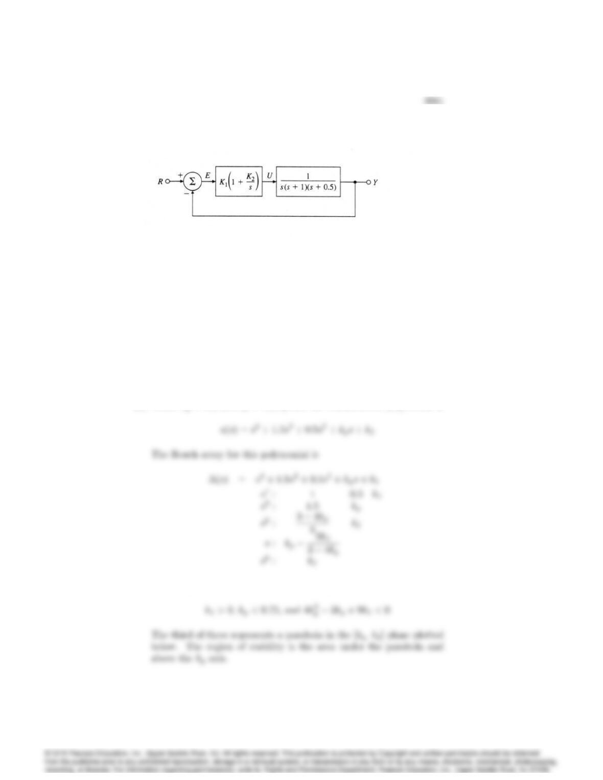
44. Consider the system in Fig. 5.63.
Figure 5.63: Feedback system for Problem 5.44
(a) Use Routh’s criterion to determine the regions in the (K1; K2)plane
for which the system is stable.
(b) Use rltool to verify your answer to part (a).
Solution:
(a) Define kp=K1and kI=K1K2and the characteristic polynomial is
For the system to be stable, it is necessary that
5082 CHAPTER 5. THE ROOT-LOCUS DESIGN METHOD
00.1 0.2 0.3 0 .4 0 .5 0 .6 0.7 0.8
0
0.01
0.03
0.05
0.07
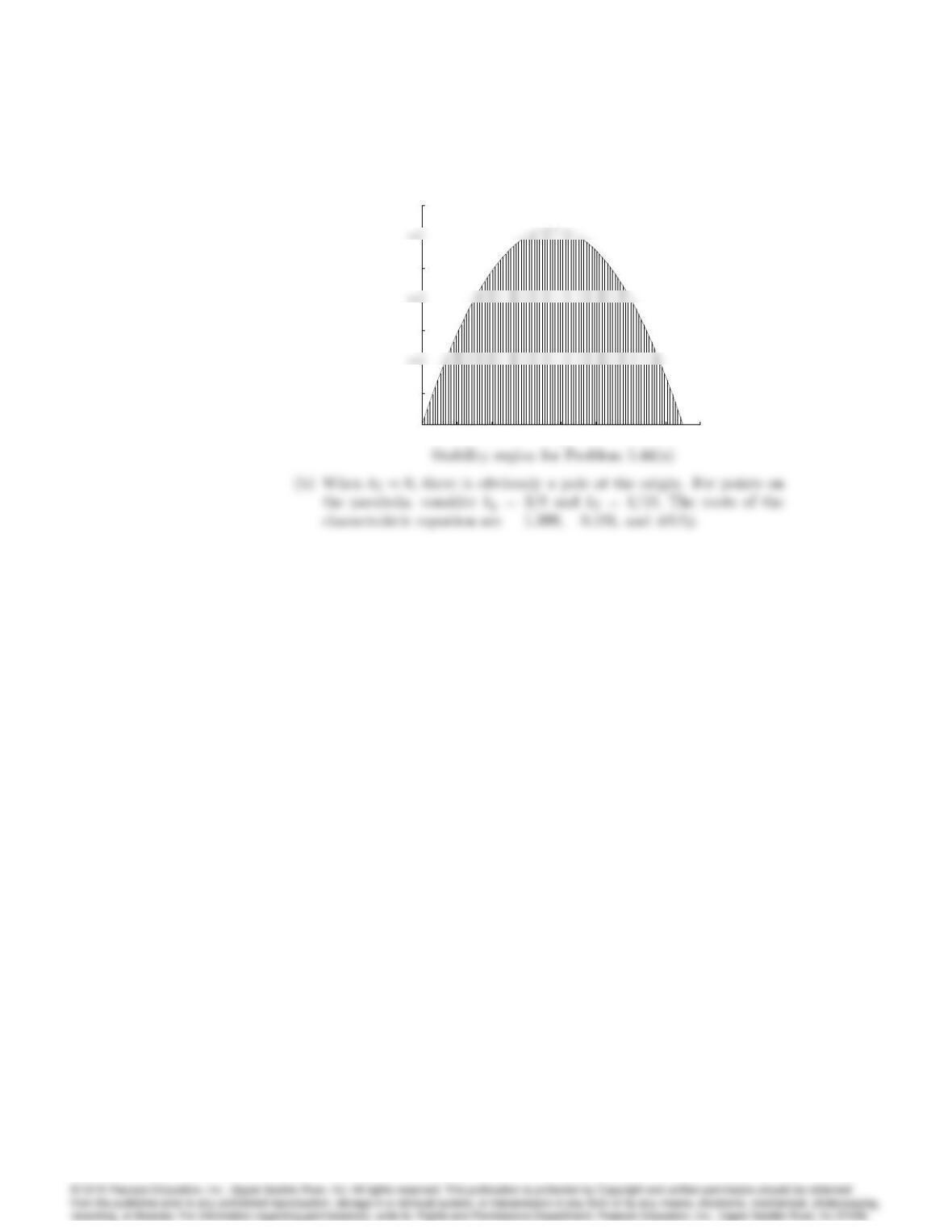
Stability region in the kp,kI plane for problem 5.43
kp
kI
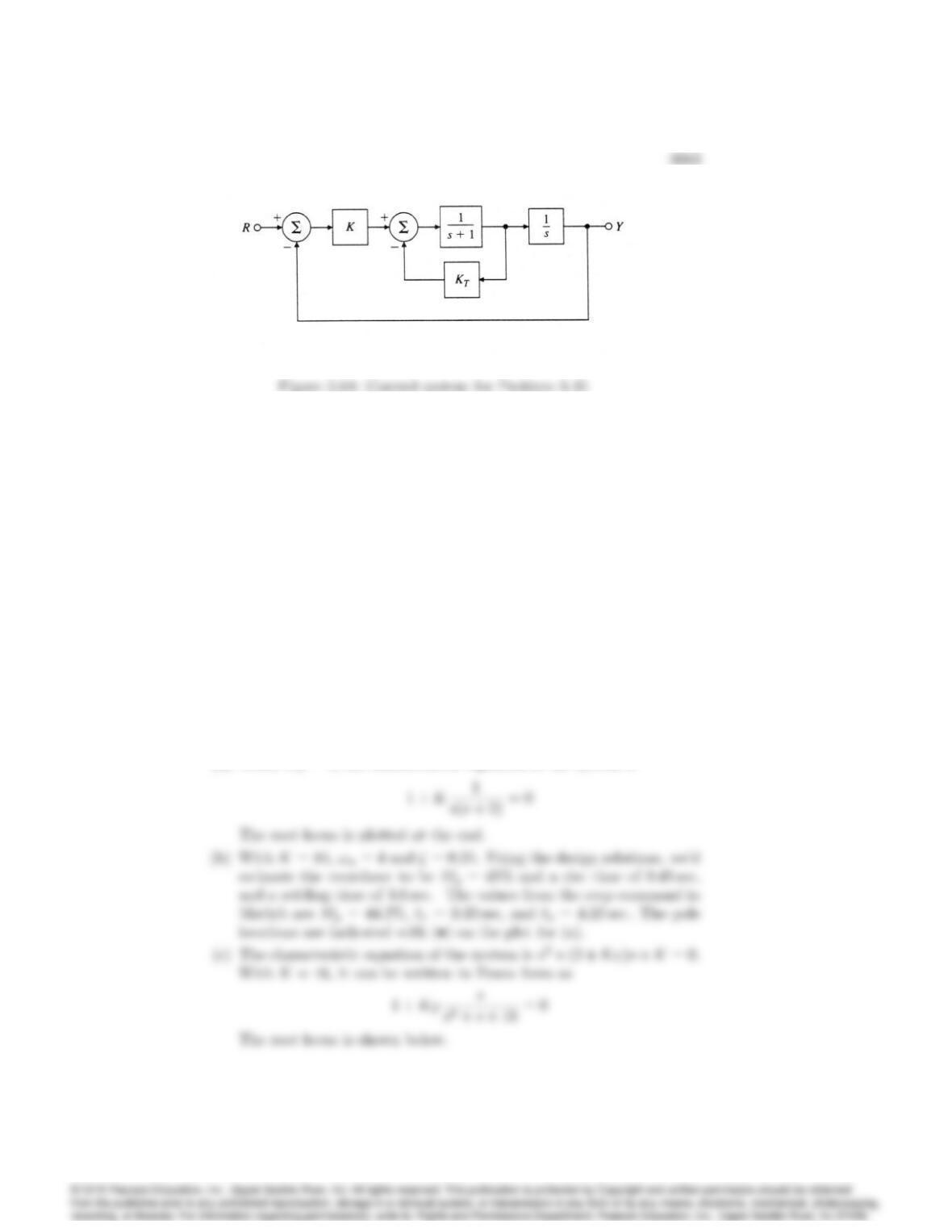
45. The block diagram of a positioning servomechanism is shown in Fig. 5.64.
(a) Sketch the root locus with respect to Kwhen no tachometer feedback
is present (KT= 0).
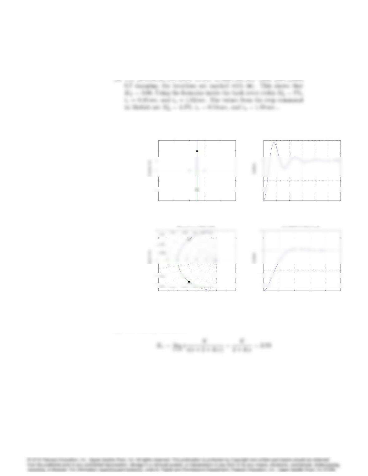
(b) Indicate the root locations corresponding to K= 16 on the locus
of part (a). For these locations, estimate the transient-response pa-
rameters tr,Mp, and ts. Compare your estimates to measurements
obtained using the step command in Matlab.
(c) For K= 16, draw the root locus with respect to KT.
(d) For K= 16 and with KTset so that Mp= 0:05(= 0:707), estimate
trand ts. Compare your estimates to the actual values of trand ts
obtained using Matlab.
(e) For the values of Kand KTin part (d), what is the velocity constant
Kvof this system?
Solution:
(a) When KT= 0, the characteristic equation of the system is
5084 CHAPTER 5. THE ROOT-LOCUS DESIGN METHOD
-6 -4 -2 0 2 4
-6
-2
4
6
Root locus f or Problem 5.45(a)
Real Axis
0 1 2 3 4 5 6
0
0.5
1.5
St ep response f or Problem 5. 45(b)
Time (sec)
-6 -5 -4 -3 -2 -1 0 1 2
-4
-1
0.160.340.50.640.76
0.985
Root locus vs KT , Problem 5.45(c)
Real Axis
I m aginar y A xis
00.5 11.5 22.5
0
0.5
st ep response f or Problem 5.45(d)
Time (sec)
Amplitude
Plots for Problem 5.45
(e) The velocity constant is
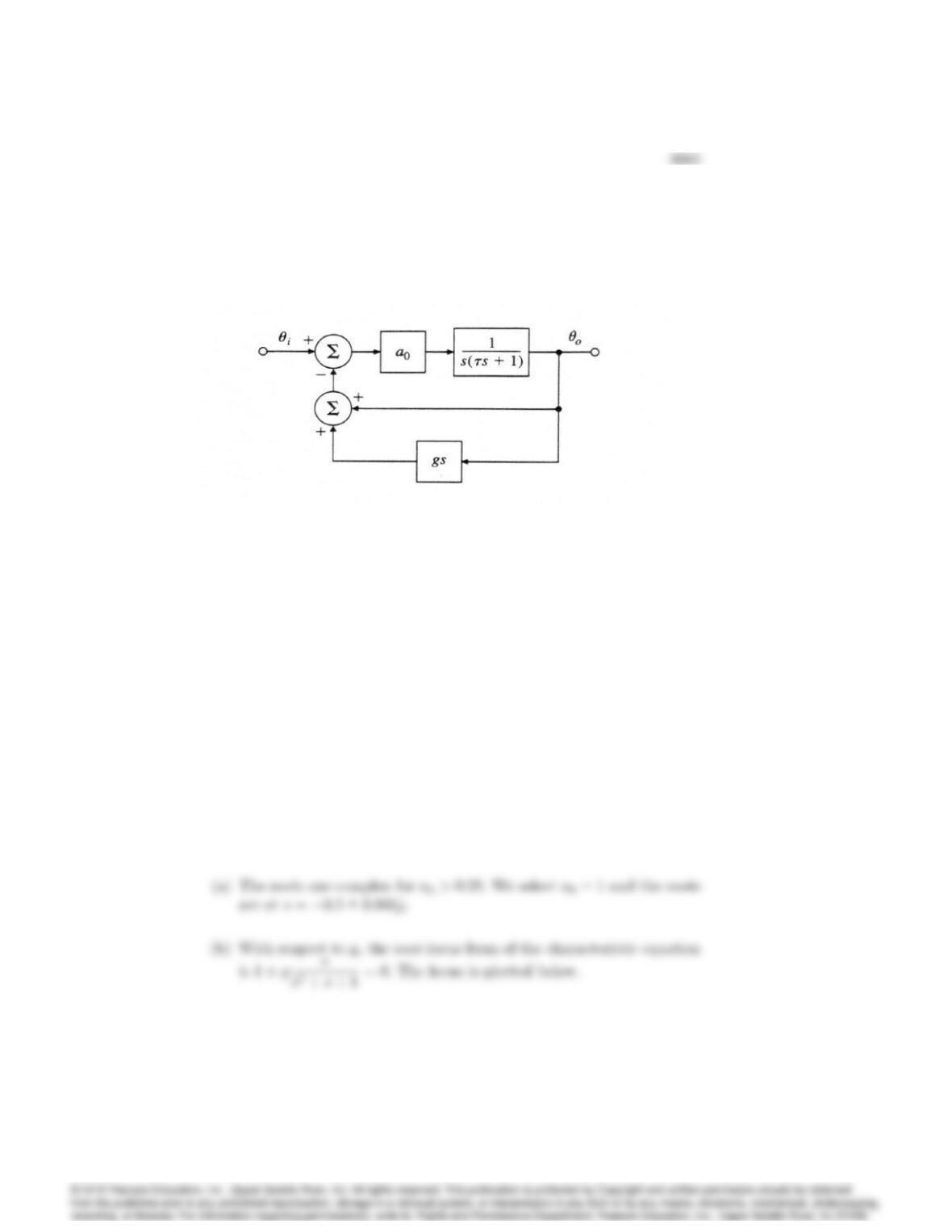
46. Consider the mechanical system shown in Fig. 5.65, where gand a0are
gains. The feedback path containing gs controls the amount of rate feed-
back. For a fixed value of a0, adjusting gcorresponds to varying the
location of a zero in the s-plane.
Figure 5.65: Control system for Problem 5.46
(a) With g= 0 and = 1, find a value for a0such that the poles are
complex.
(b) Fix a0at this value, and construct a root locus that demonstrates
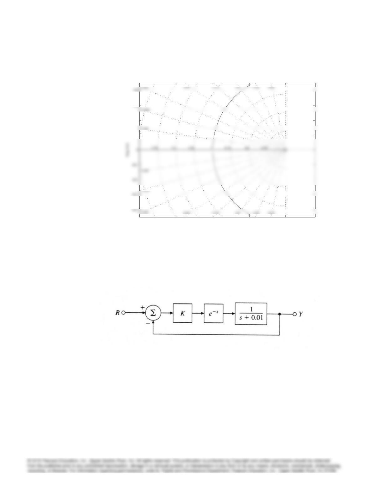
the effect of varying g.
Solution:
5086 CHAPTER 5. THE ROOT-LOCUS DESIGN METHOD
Rootlocus for problem 5.46
Real Axis
-2 –1.5 -1 -0.5 0
0.2
0.4
0.6
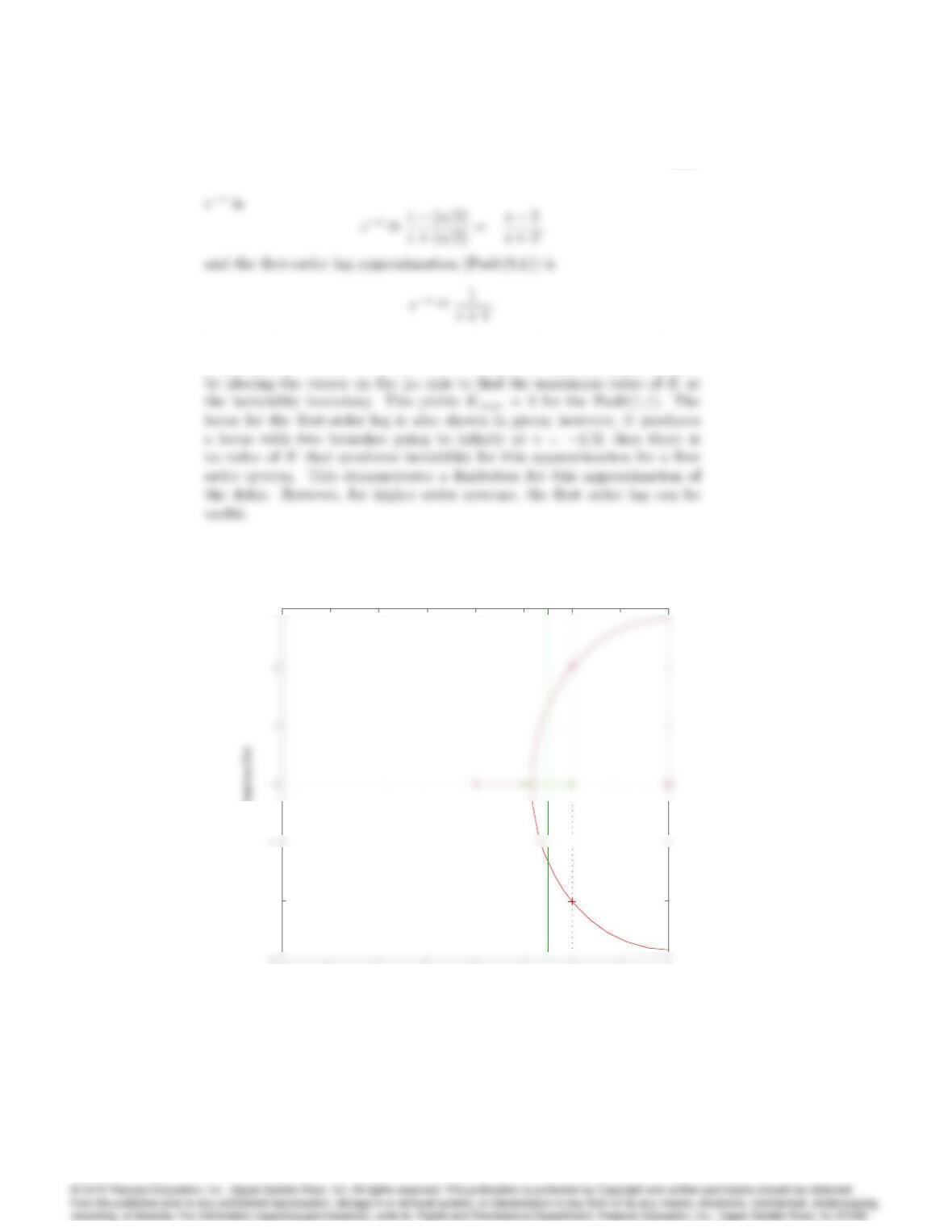
47. Sketch the root locus with respect to Kfor the system in Fig. 5.66 using
the Padé(1,1) approximation and the first-order lag approximation. For
both approximations, what is the range of values of Kfor which the system
is unstable?(Note: The material to answer this question is contained in
Appendix W5.6.3 discussed in www.FPE7e.com.)
Figure 5.66: Control system for Problem 5.47
Solution:
Matlab cannot directly plot a root locus for a transcendental function.
From the Appendix W5.6.3, we see that the Padé(1,1) approximation for
5087
With the Padé(1,1) approximation, a locus valid for small values of scan
be plotted, as shown below by the red curve. The rlocfind routine is used
-6 -5 -4 -3 -2 -1 0 1 2
-2
3
Root loci f or problem 5.46 with the (1,1)and (0,1) Pade aproximates
Real Axis
Imaginary Axis
Solutions for Problem 5.47
48. Prove that the plant G(s) = 1=s3cannot be made unconditionally stable
if pole cancellation is forbidden.
Solution:
The angles of departure from a triple pole are 180and 60for the
5089
49. For the equation 1 + KG(s)where,
G(s) = 1
s(s+p)[(s+ 1)2+ 4];
use Matlab to examine the root locus as a function of Kfor pin the range
from p= 1 to p= 10, making sure to include the point p= 2.
Solution:
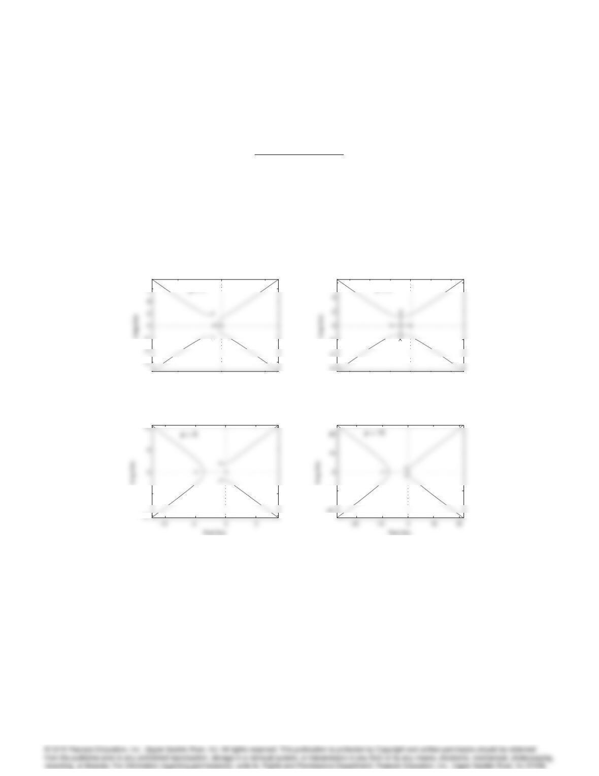
The root loci for four values are given in the figure. The point is that the
locus for p= 2 has multiple roots at a complex value of s:
Problem 5.49
Real Axis
-5 0 5
-2
6
Problem 5.49
Real Axis
-6 -4 -2 0 2 4
-2
6
p = 2
Problem 5.49
-5
Problem 5.49
–10
Solutions for Problem 5.49