5020 CHAPTER 5. THE ROOT-LOCUS DESIGN METHOD
12. Sketch the root locus for the characteristic equation of the system for
which
L(s) = (s+ 2)
s2(s+ 5);
and determine the value of the root-locus gain for which the complex con-
jugate poles have the maximum damping ratio. What is the approximate
value of the damping?
Solution:
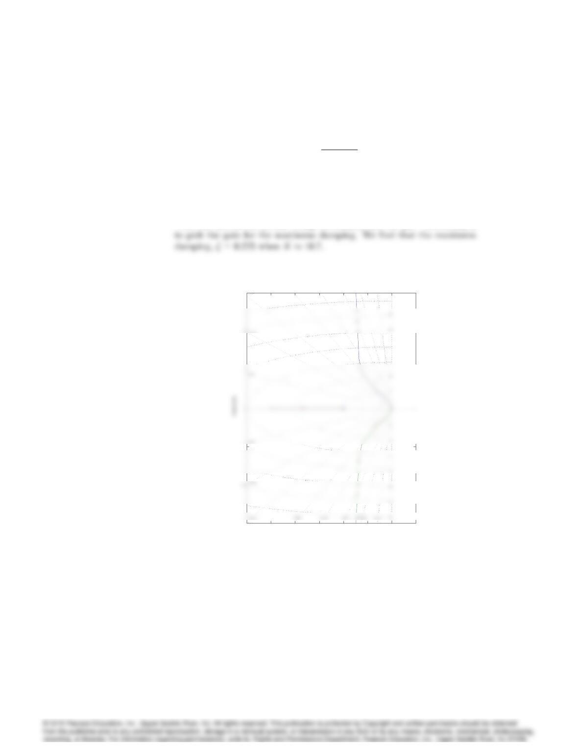
Plot the system on Matlab using rlocus(sys), and use [K]= rlocfind(sys)
-6 -5 -4 -3 -2 -1 0 1
-15
-5
15
6
8
14
0.040.0850.130.190.26
0.38
0.52
Root Loc us
Real Axis
Root locus with 0.275 damping marked
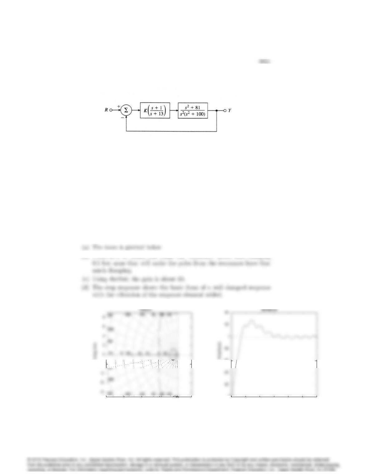
13. For the system in Fig. 5.47,
Figure 5.47: Feedback system for Problem 5.13
(a) Find the locus of closed-loop roots with respect to K.
(b) Is there a value of Kthat will cause all roots to have a damping ratio
greater than 0:5?
(c) Find the values of Kthat yield closed-loop poles with the damping
ratio = 0:707.
(d) Use Matlab to plot the response of the resulting design to a reference
step.
Solution:
(b) There is a Kwhich will make the ’dominant’ poles have damping
Real Axis
– 20 – 15 – 10 -5 0
-2
Time (sec)
0 1 2 3 4 5 6
0
0.6

Root locus and step response for Problem 5.13
5023
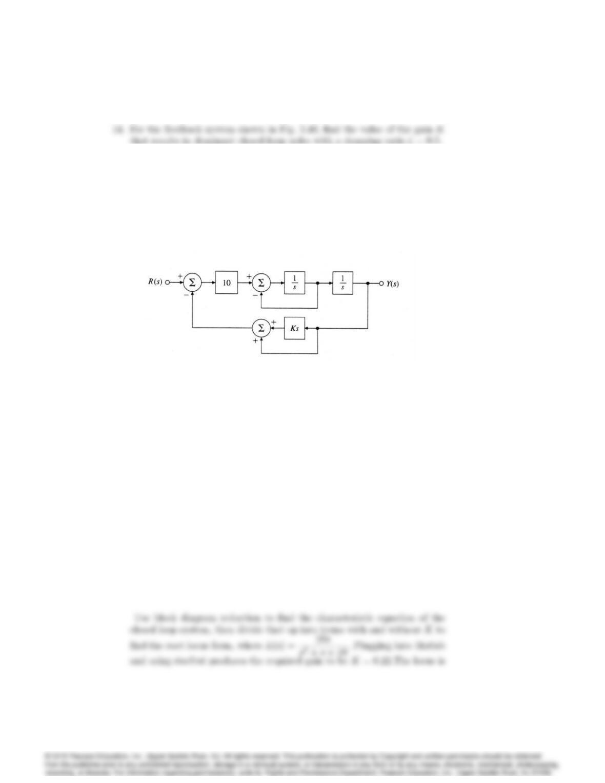
Figure 5.48: Feedback system for Problem 5.14
Solution:
5024 CHAPTER 5. THE ROOT-LOCUS DESIGN METHOD
-6 -5 -4 -3 -2 -1 0 1
-4
2
4
0.140.30.440.580.72
0.84
R oot Locus
R eal Axis
Imaginary Axi s
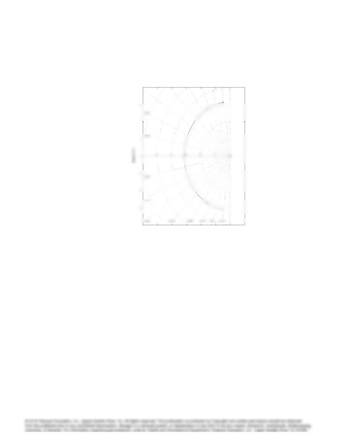
Root locus with 0.5 damping marked

5025
Problems and solutions for Section 5.3
15. A simplified model of the longitudinal motion of a certain helicopter near
hover has the transfer function
G(s) = 9:8(s20:5s+ 6:3)
(s+ 0:66)(s20:24s+ 0:15):
and the characteristic equation 1 + Dc(s)G(s) = 0. Let Dc(s) = kpat
first.
(a) Compute the departure and arrival angles at the complex poles and
zeros.
(b) Sketch the root locus for this system for parameter K= 9:8kp. Use
axes –4x4;3y3;
(c) Verify your answer using Matlab. Use the command axis([-4 4 -3 3])
to get the right scales.
(d) Suggest a practical (at least as many poles as zeros) alternative com-
pensation Dc(s)which will at least result in a stable system.
Solution:
(b) (c)
-4 -3 -2 -1 0 1 2 3 4
-3
3
Root Locus
Rea l A x is
Problem 5.15(b)(c)

5026 CHAPTER 5. THE ROOT-LOCUS DESIGN METHOD
(d) For this problem a double lead is needed to bring the roots into the
left half-plane. The plot shows the rootlocus for control for. Let
Dc(s) = (s+:66)(s+:33)
(s+ 5)2:
-4 -3 -2 -1 0 1 2 3 4
-2
3
Root Locus
Real A x is
Imaginary Axis
Problem 5.15(d)
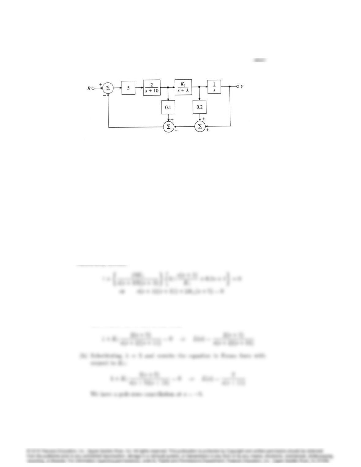
Figure 5.49: Control system for Problem 5.16
16. For the system given in Fig. 5.49,
(a) Plot the root locus of the characteristic equation as the parameter
K1is varied from 0to 1with = 2. Give the corresponding L(s);
a(s);and b(s):
(b) Repeat part (a) with = 5. Is there anything special about this
value?
(c) Repeat part (a) for fixed K1= 2 with the parameter K=varying
from 0to 1.
Solution:
Use block diagram reduction to find the characteristic equation of the
closed-loop system:
The root locus for each part is attached at the end.
(a) Substituting = 2 and divide the equation above up into terms with
and without K1to find Evans form:
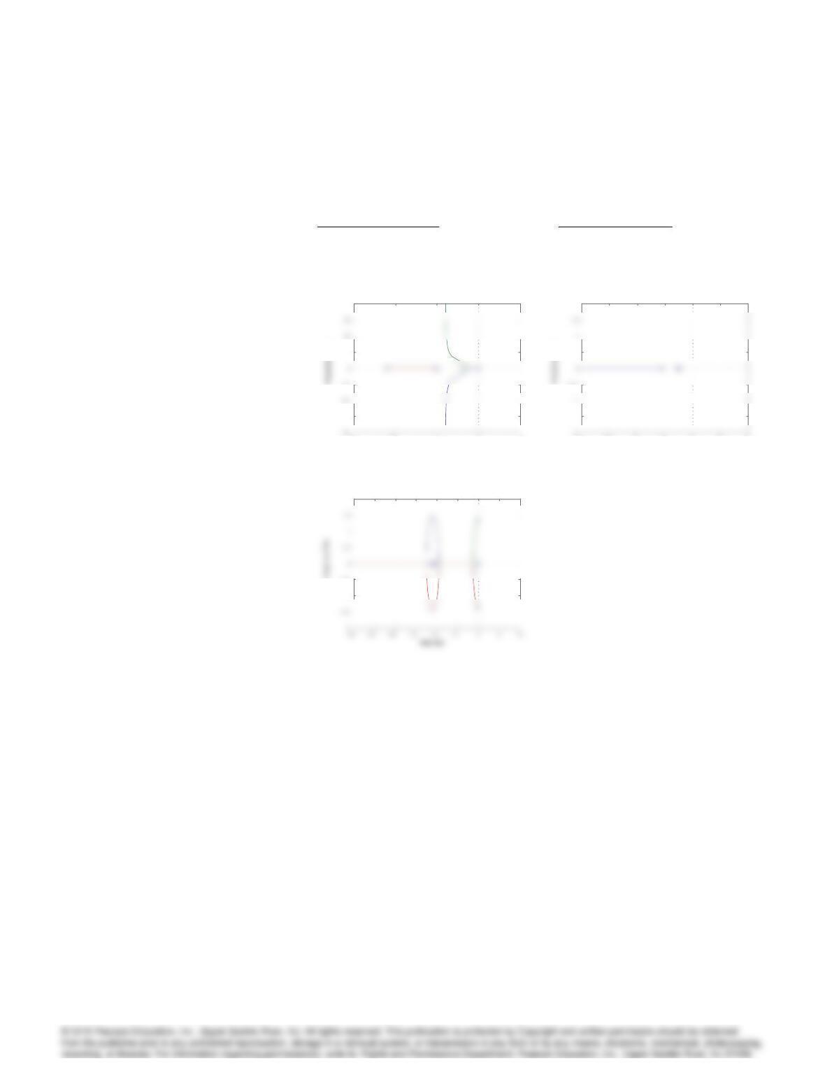
5028 CHAPTER 5. THE ROOT-LOCUS DESIGN METHOD
(c) Substituting K1= 2 and divide the characteristic equation up into
terms with and without to find Evans form:
1 + s(s+ 11)
s2(s+ 11) + 4(s+ 5) = 0 )L(s) = s(s+ 11)
s3+ 11s2+ 4s+ 20
–15 –10 -5 0 5
–30
–10
10
40
plot a
Real Axis
–40 – 30 – 20 –10 010 20
-1.5
-0.5
0.5
2
plot b
Real Axis
-1
-0.5
2
plot c
Imaginary Axis
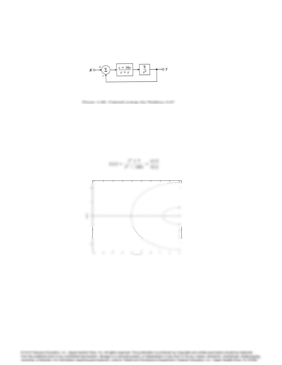
Solution for Problem 5.16
5029
17. For the system shown in Fig. 5.50, determine the characteristic equation
and sketch the root locus of it with respect to positive values of the pa-
rameter c. Give L(s),a(s);and b(s)and be sure to show with arrows the
direction in which cincreases on the locus.
Solution:
Root Locus
Real Ax is
-5
Solution for Problem 5.17
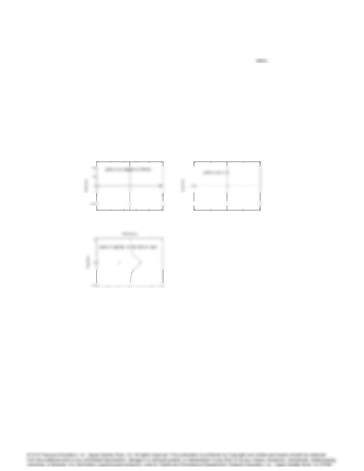
18. Suppose you are given a system with the transfer function
L(s) = (s+z)
(s+p)2;
where zand pare real and z > p. Show that the root locus for 1+KL(s) =
0with respect to Kis a circle centered at zwith radius given by
r= (zp):
Hint: Assume s+z=rej and show that L(s)is real and negative for
real under this assumption.
Solution:
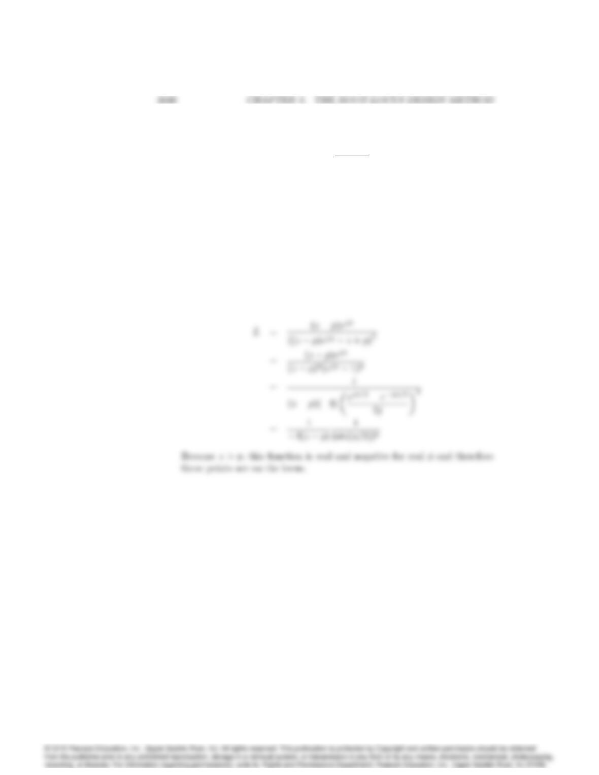
Assume s+z= (zp)ej. Then L(s)can be written as:
19. The loop transmission of a system has two poles at s=1and a zero
at s=2. There is a third real-axis pole plocated somewhere to the
left of the zero. Several different root loci are possible, depending on the
exact location of the third pole. The extreme cases occur when the pole
is located at infinity or when it is located at s=2. Give values for p
and sketch the three distinct types of loci.
Solution:
Root Locus
Real Axis
–100 –80 –60 –40 –20 0
–10
Root Locus
Real Axis
-2 –1.5 -1 -0.5 0
–0.5
0.5
Real Axis
-3 –2.5 -2 -1.5 -1 –0.5 0
Solution for Problem 5.19
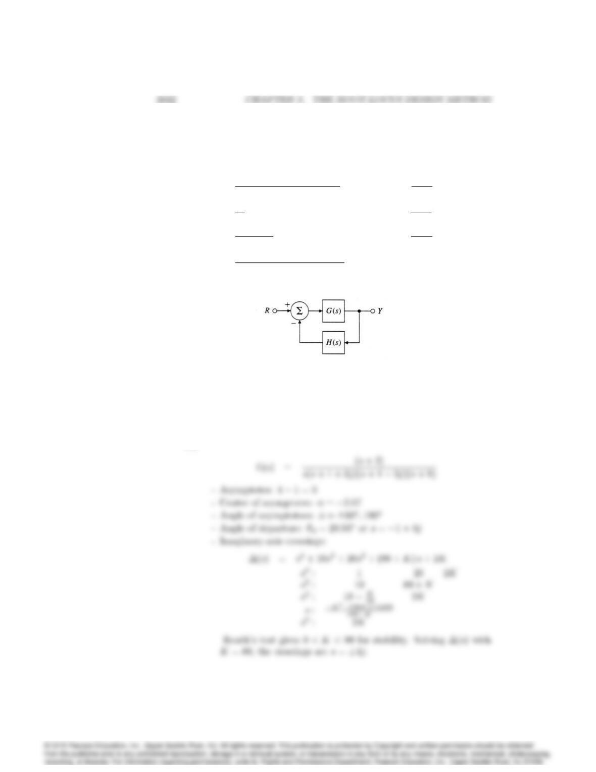
20. For the feedback configuration of Fig. 5.51, use asymptotes, center of
asymptotes, angles of departure and arrival, and the Routh array to sketch
root loci for the characteristic equations of the listed feedback control
systems versus the parameter K: Use Matlab to verify your results.
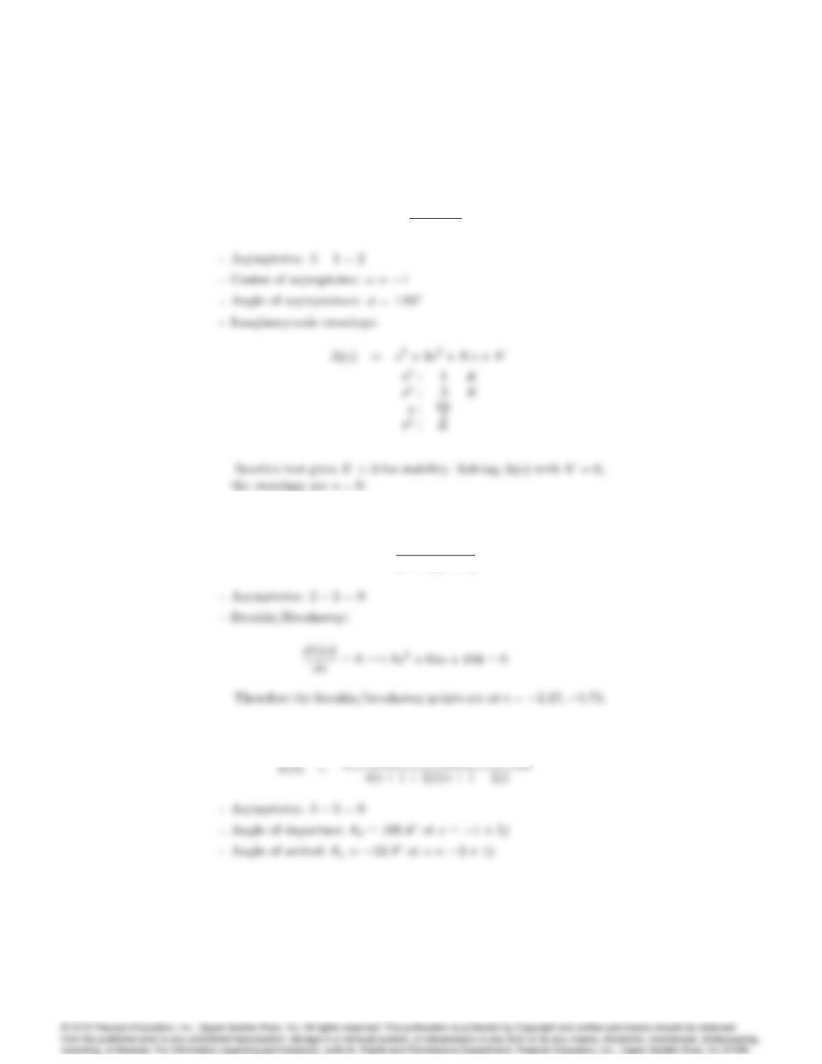
(a) G(s) = K
s(s+ 1 + 3j)(s+ 1 3j); H(s) = s+ 2
s+ 8
(b) G(s) = K
s2; H(s) = s+ 1
s+ 3
(c) G(s) = K(s+ 5)
(s+ 1) ; H(s) = s+ 7
s+ 3
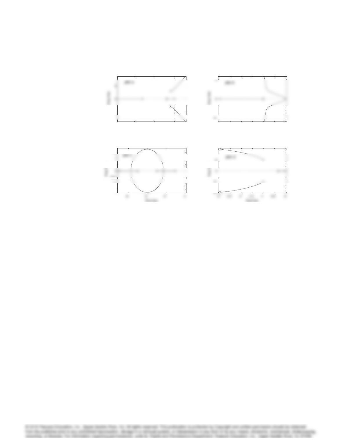
(d) G(s) = K(s+ 3 + 4j)(s+ 3 4j)
s(s+ 1 + 2j)(s+ 1 2j); H(s) = 1 + 3s
Figure 5.51: Feedback system for Problem 5.20
Solution:
The root locus for each part is attached at the end.
(a)
5033
(b)
L(s) = (s+ 1)
s2(s+ 3)
(c)
L(s) = (s+ 5)(s+ 7)
(s+ 1)(s+ 3)
(d)
5034 CHAPTER 5. THE ROOT-LOCUS DESIGN METHOD
Root Locus
Real Axis
–10 -5 0
-5
Root Locus
Real Axis
-3 –2.5 -2 –1.5 -1 -0.5 0
Root Locus
–1.5
-1
–0.5
0.5
1.5
Root Locus
4
Solution for Problem 5.20
5035
Figure 5.52: Feedback system for Problem 5.21
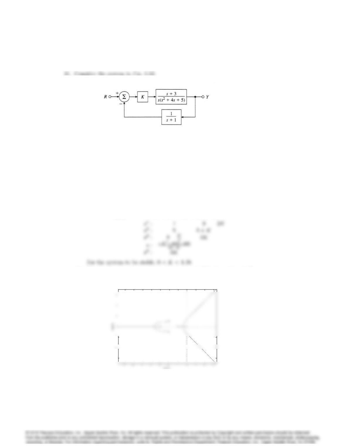
(a) Using Routh’s stability criterion, determine all values of Kfor which
the system is stable.
(b) Use Matlab to find the root locus versus K. Find the values for K
at imaginary-axis crossings.
Solution:
(a)
(s) = s4+ 5s3+ 9s2+ (5 + K)s+ 3K
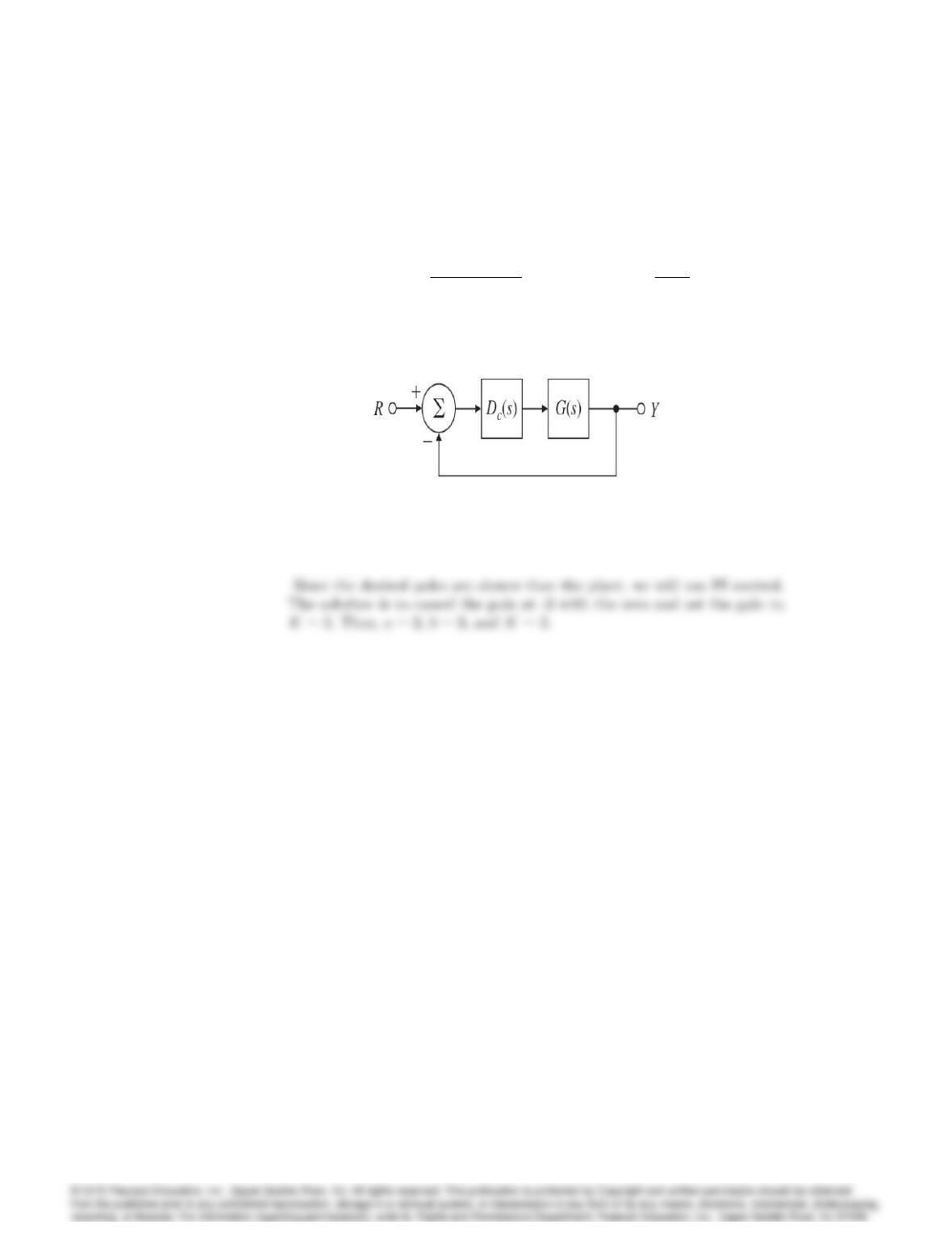
(b) The imaginary axis crossings are at s=1:38jwhen K= 4:49.
Root locus is shown below.
Root Locus
-6
-2
Root locus for Problem 5.21
5036 CHAPTER 5. THE ROOT-LOCUS DESIGN METHOD
Problems and solutions for Section 5.4
22. Let
G(s) = 1
(s+ 2)(s+ 3) and Dc(s) = Ks+a
s+b:
Using root-locus techniques, find values for the parameters a; b, and Kof
the compensation Dc(s)that will produce closed-loop poles at s=1j
for the system shown in Fig. 5.53.
Figure 5.53: Unity feedback system for Problems 5.22, 5.28, and 5.33
Solution:
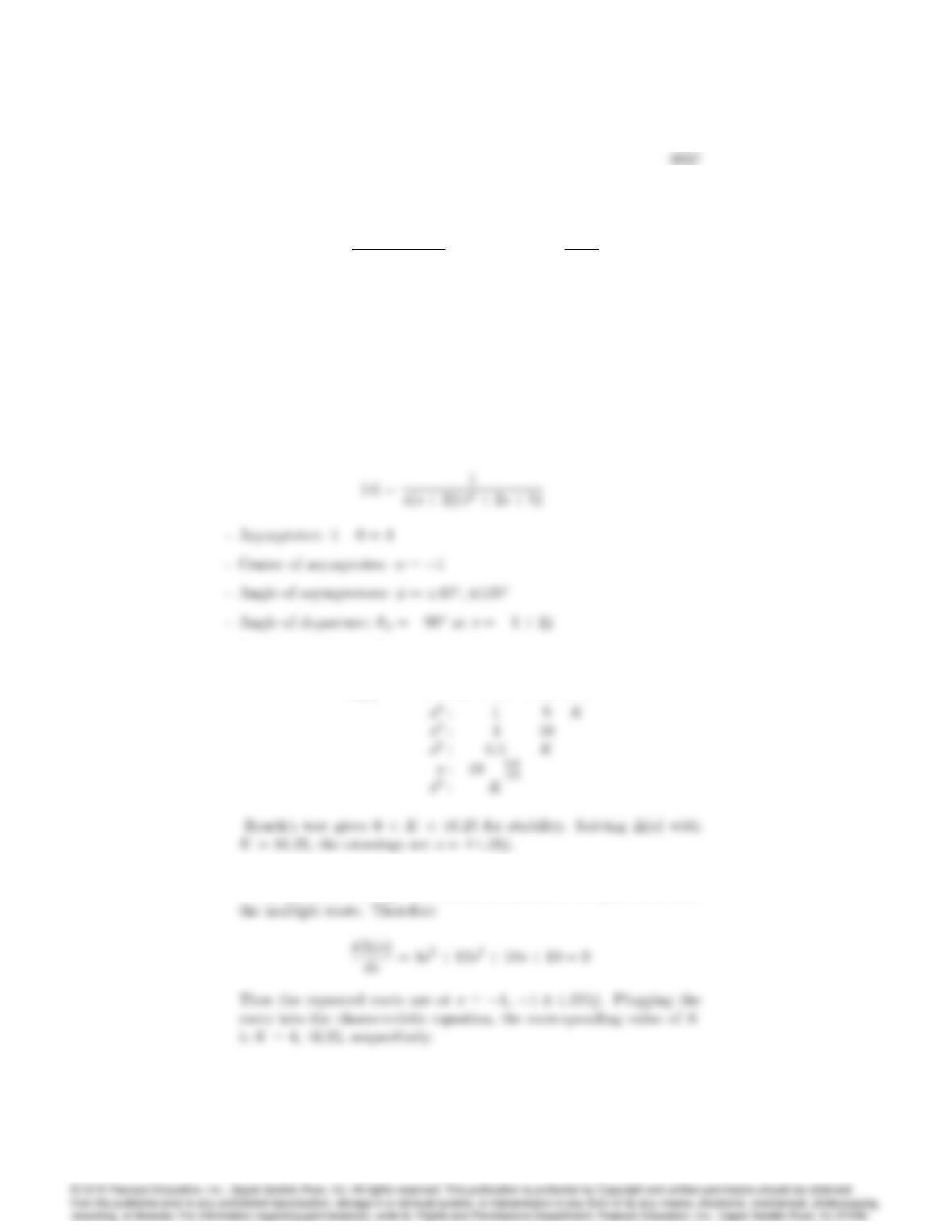
23. Suppose that in Fig. 5.53,
G(s) = 1
s(s2+ 2s+ 5) and Dc(s) = K
s+ 2:
Without using Matlab, sketch the root locus with respect to Kof the
characteristic equation for the closed-loop system, paying particular at-
tention to points that generate multiple roots. Find the value of Kat
that point, state what the location of the multiple roots is, and how many
multiple roots there are.
Solution:
The root locus for the system is attached at the end.
– Imaginary-axis crossings:
(s) = s4+ 4s3+ 9s2+ 10s+K
– Location of multiple roots:
If a polynomial has repeated roots, its derivative is equal to zero at

5038 CHAPTER 5. THE ROOT-LOCUS DESIGN METHOD
-4 -3 -2 -1 0 1 2
-3
-1
Real Axis
Root locus for Problem 5.23
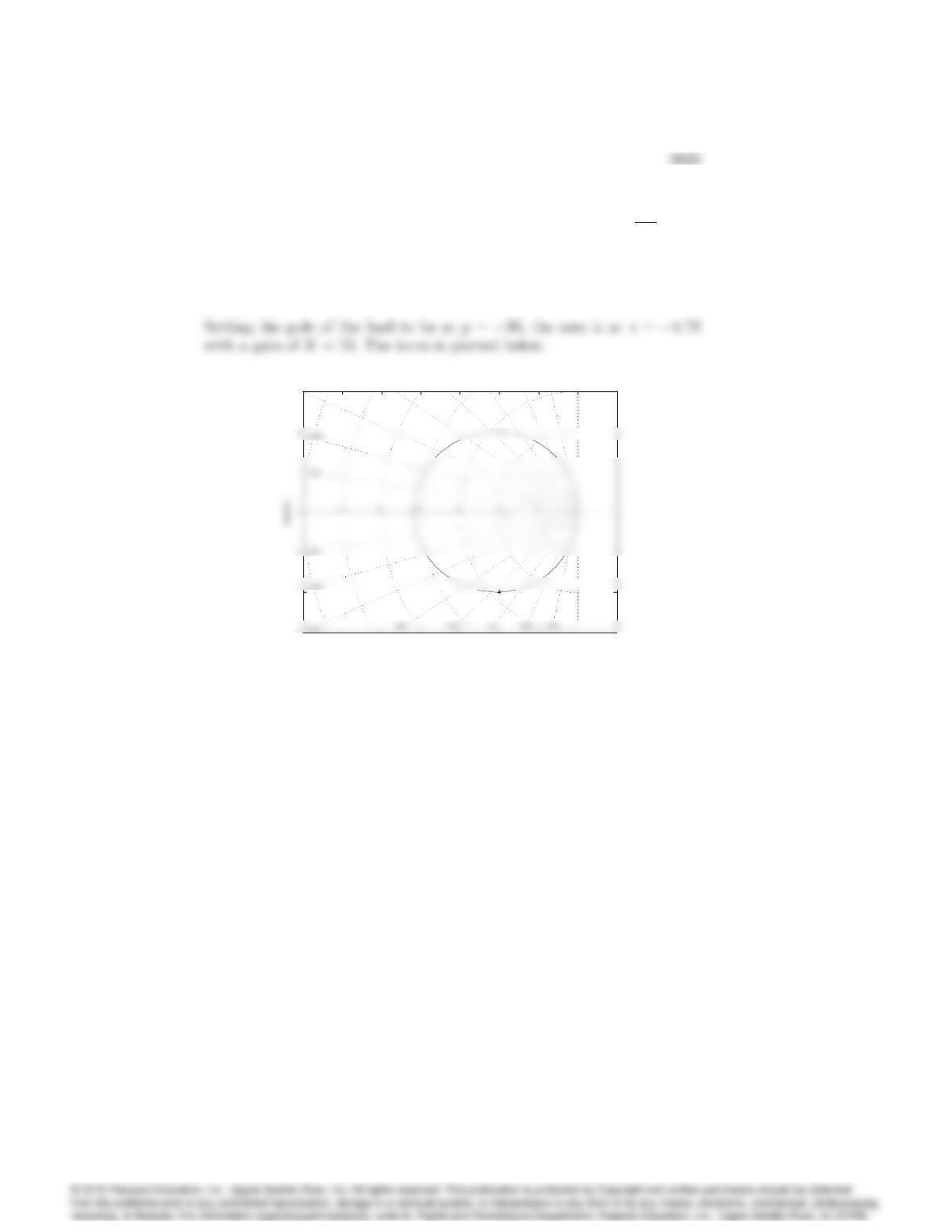
24. Suppose the unity feedback system of Fig. 5.53 has an open-loop plant
given by G(s) = 1=s2. Design a lead compensation Dc(s) = Ks+z
s+pto be
added in series with the plant so that the dominant poles of the closed-loop
system are located at s=22j.
Solution:
Root Locus
Real Axis
-7 -6 -5 -4 -3 -2 -1 0 1
-3
-2
3
0.92 0.84 0.74 0 .6 0.42 0.22
Root locus for Problem 5.24