Operating Systems Chapter 4 Homework Let u2 be the signal coupling systems 1 and 2

4020 CHAPTER 4. CHAPTER 4: A FIRST ANALYSIS OF FEEDBACK

(s)is the characteristic polynomial, same as in (i) (denominator in

(i)).

yss = [lim

s!0s:W2(s):sl1]Qip1i

Qiz1i

Type `1

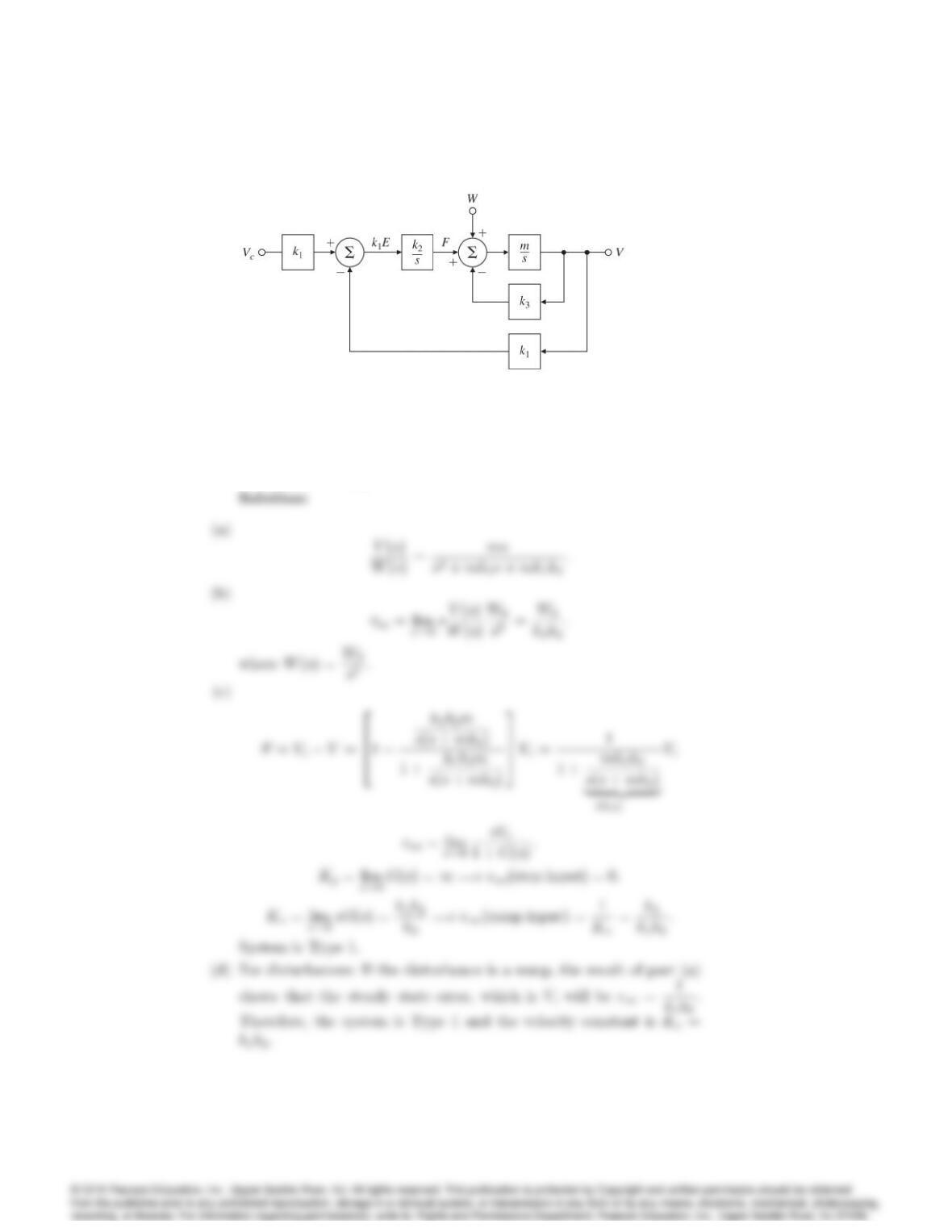
18. One possible representation of an automobile speed-control system with

integral control is shown in Fig. 4.33.

(a) With a zero reference velocity input (vc= 0), find the transfer func-

tion relating the output speed vto the wind disturbance w.

(b) What is the steady-state response of vif wis a unit ramp function?

(c) What type is this system in relation to reference inputs? What is the

value of the corresponding error constant?

4021

Figure 4.33: System using integral control

(d) What is the type and corresponding error constant of this system in

relation to tracking the disturbance w?

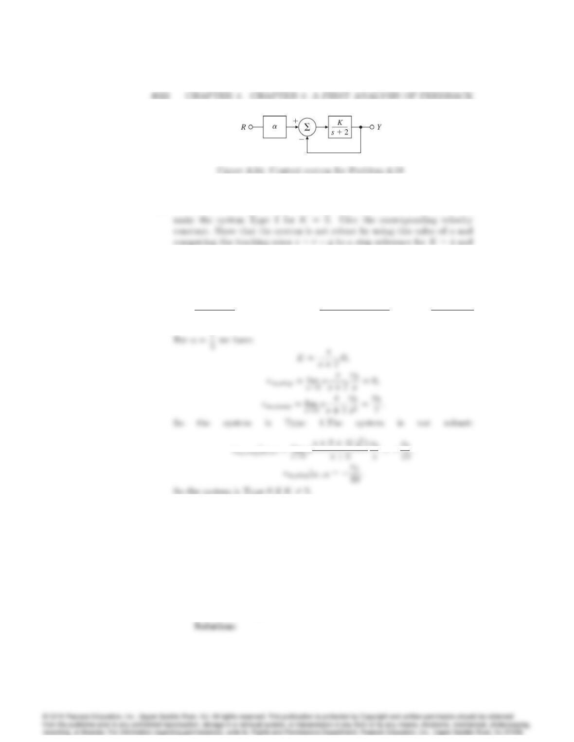
19. For the feedback system shown in Fig. 4.34, find the value of that will

K= 6.

Solution:

Y=KR

s+ 2 + KE=RY=s+ 2 + K(1 )

s+ 2 + KRK=5

=s+ 7 5

s+ 7 R:

5)

20. Suppose you are given the system depicted in Fig. 4.35(a), where the plant

parameter ais subject to variations.

(a) Find G(s)so that the system shown in Fig. 4.35(b) has the same

transfer function from rto yas the system in Fig. 4.35(a).

(b) Assume that a= 1 is the nominal value of the plant parameter.

What is the system type and the error constant in this case?

(c) Now assume that a= 1 + a, where a is some perturbation to the

plant parameter. What is the system type and the error constant for

the perturbed system?

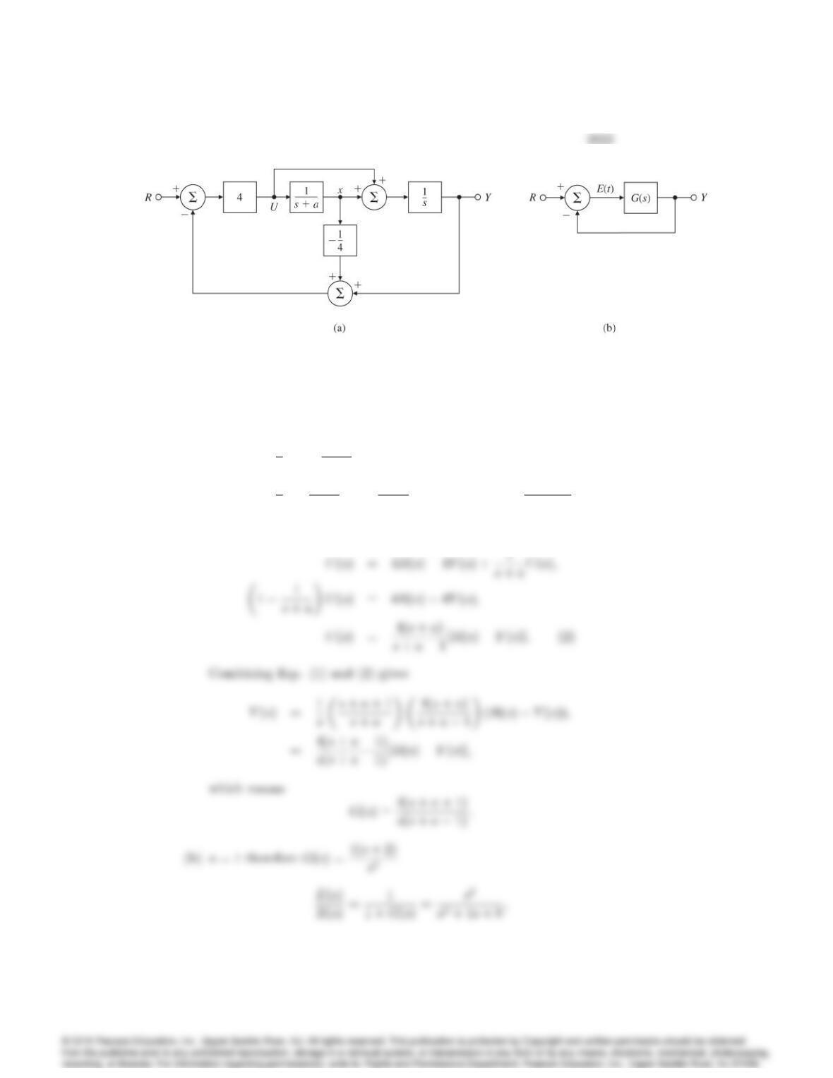
Figure 4.35: Control system for Problem 4.20

(a)

Y(s) = 1

s1 + 1

s+aU(s);

=1

s1 + 1

s+a1 + 1

s+a4(R(s)Y(s) + 1

4(s+a)U(s)):(1)

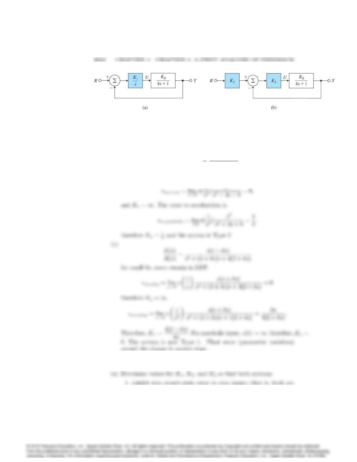
Figure 4.36: Two feedback systems for Problem 4.21

roots are in LHP so we can use the FVT,

ess;step = lim

!0s(1

s)s2

s2+ 4s+ 8 = 0;

therefore Kp=1

21. Two feedback systems are shown in Fig. 4.36.

Type 1), and

4025

ii. whose static velocity error constant Kv= 1 when K0= 1.

(b) Suppose K0undergoes a small perturbation: K0!K0+K0. What

effect does this have on the system type in each case? Which system

has a type which is robust? Which system do you think would be

preferred?

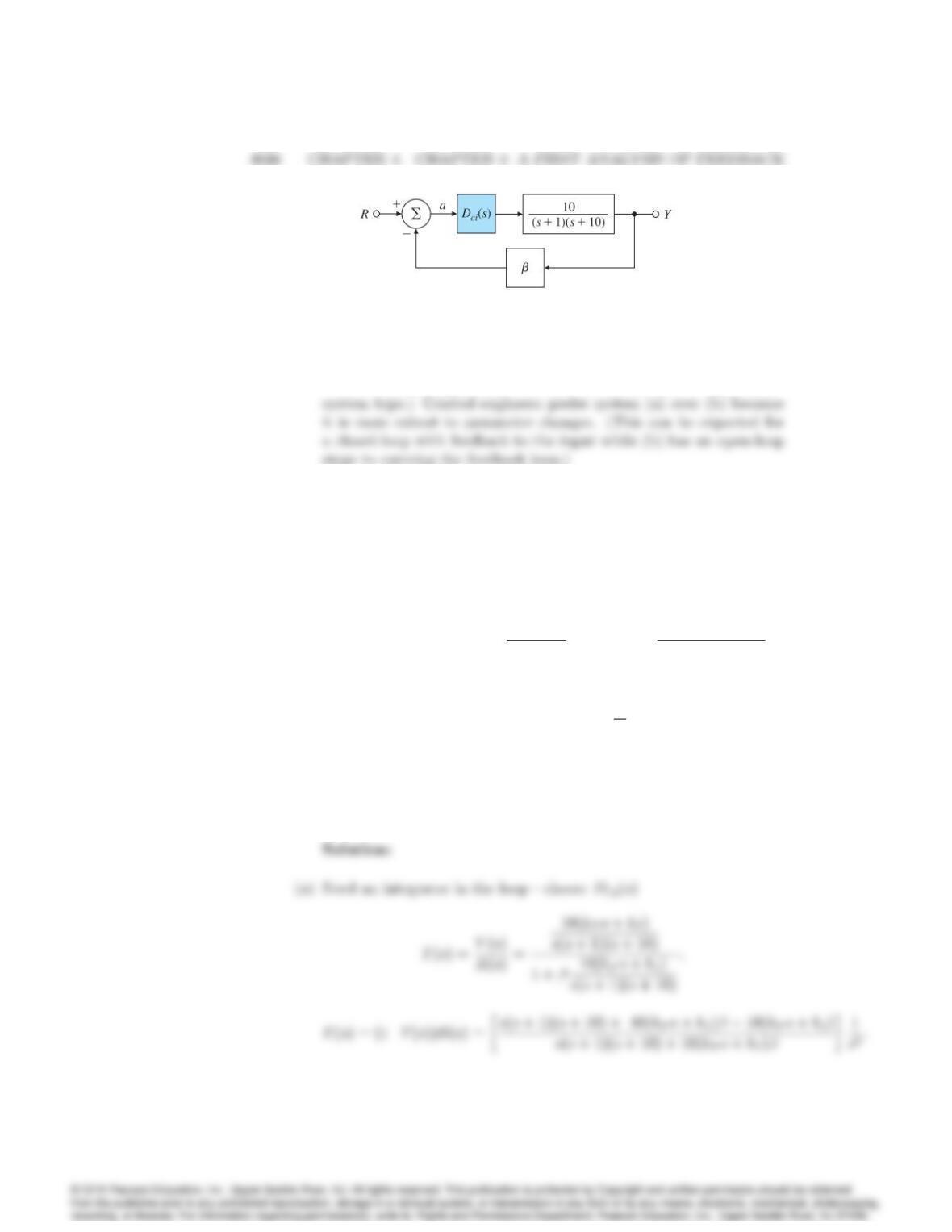
Figure 4.37: Control system for Problem 4.22

Thus the system type of System (b) is not robust (it is a “calibrated”

22. You are given the system shown in Fig. 4.37, where the feedback gain 

is subject to variations. You are to design a controller for this system so

that the output y(t)accurately tracks the reference input r(t).

(a) Let = 1. You are given the following three options for the controller

Dci(s):

Dc1(s) = kP; Dc2(s) = kPs+kI

s; Dc3(s) = kPs2+kIs+k2

s2:

Choose the controller (including particular values for the controller

constants) that will result in a Type 1 system with a steady-state

error to a unit reference ramp of less than 1

10 .

(b) Next, suppose that there is some attenuation in the feedback path

that is modeled by = 0:9. Find the steady-state error due to a

ramp input for your choice of Dci(s)in part (a).

(c) If = 0:9, what is the system type for part (b)? What are the values

of the appropriate error constant?

Type 1.

(c) Try R(s) = 1

s

s(s+ 1)(s+ 10) kPskI

23. Consider the system shown in Fig. 4.38.

(a) Find the transfer function from the reference input to the tracking

error.

(b) For this system to respond to inputs of the form r(t) = tn1(t)(where

n < q) with zero steady-state error, what constraint is placed on the

open-loop poles p1; p2; ; pq?

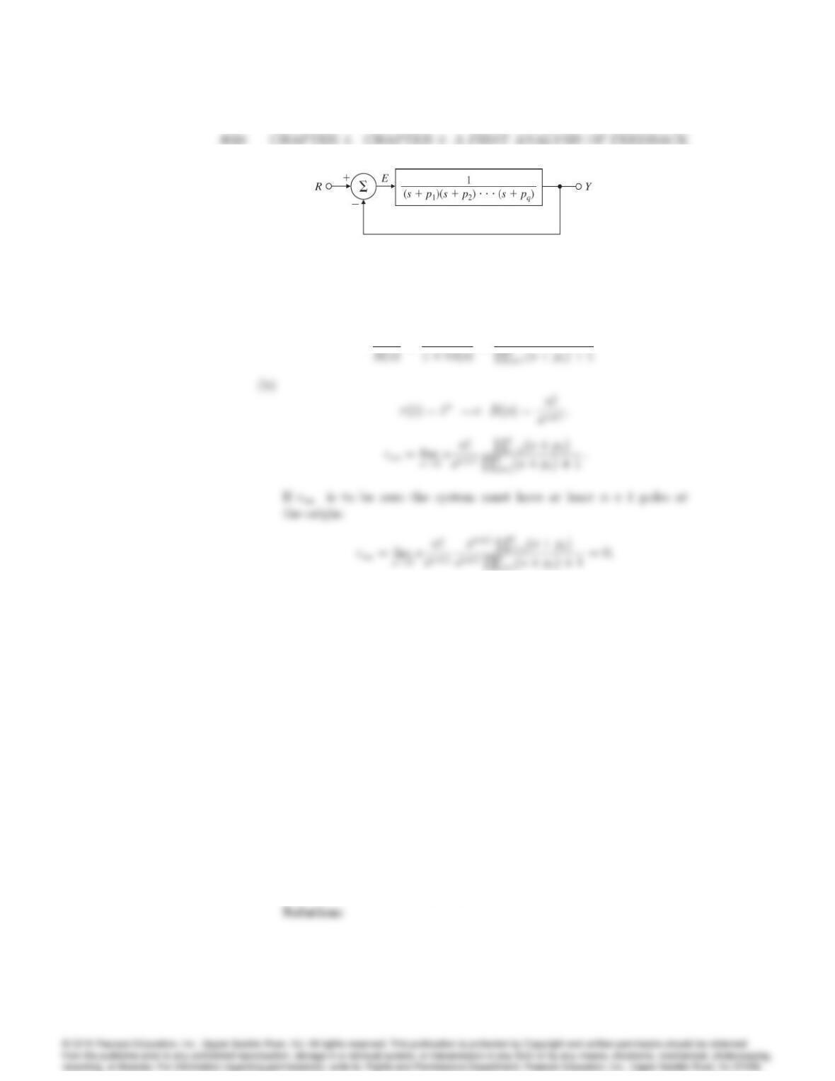
Figure 4.38: Control system for Problem 4.23

(a)

E(s)

i=1(s+pi)

Qq

24. Consider the system shown in Figure 4.39.

(a) Compute the transfer function from R(s)to E(s)and determine the

steady-state error (ess) for a unit step reference input signal, and a

unit ramp reference input signal.

(b) Determine the locations of the closed-loop poles of the system.

(c) Select the system parameters (k,kp,kI) such that the closed-loop

system has damping coefficient = 0:707 and !n= 1 What percent

overshoot would you expect in y(t)for unit step reference input?

(d) Find the tracking error signal as a function of time, e(t), if the refer-

ence input to the system, r(t), is a unit ramp.

(e) How can we select the PI controller parameters (kp,kI) to ensure

that the amplitude of the transient tracking error, je(t)j, from part

(d) is small ?

(f) What is the transient behavior of the tracking error, e(t), for a unit

ramp reference input if the magnitude of the integral gain, kI, is very

large? Does the unit ramp response have an overshoot in that case?

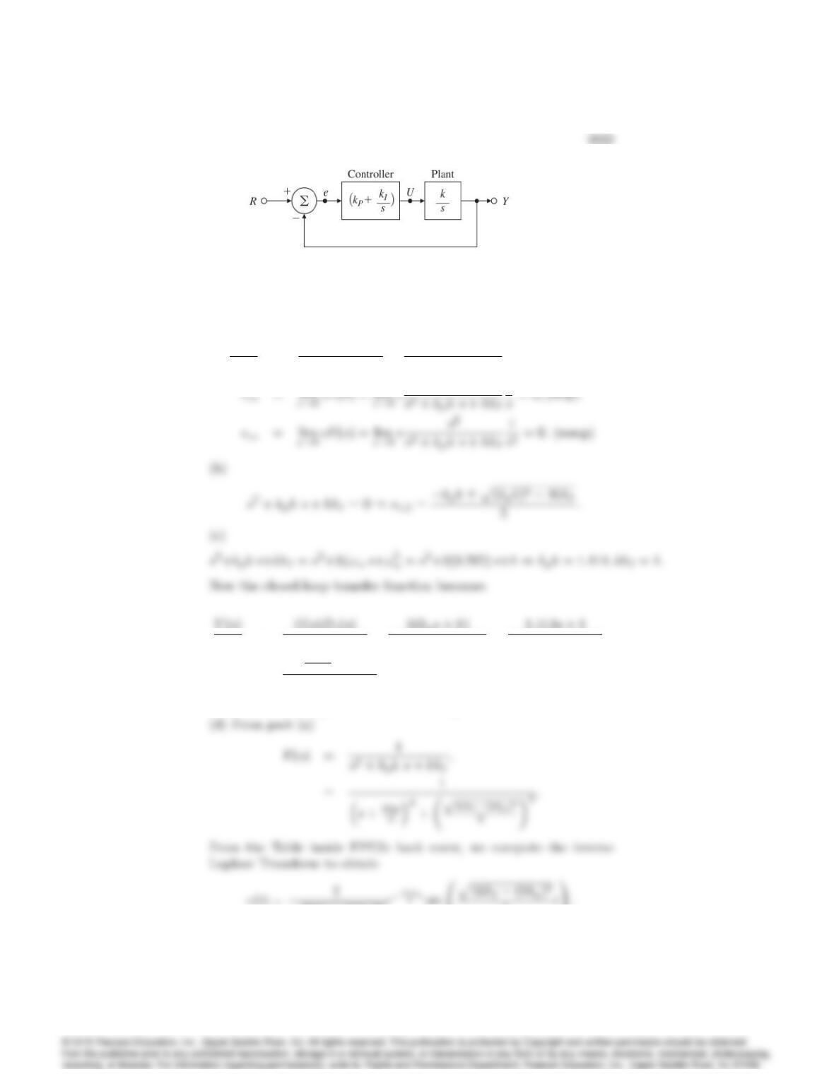
Figure 4.39: Control system diagram for Problem 4.24

(a)

E(s)

R(s)=1

1 + G(s)Dc(s)=s2

s2+kpk s +kkI

:

1

R(s)=G(s)Dc(s)

1 + G(s)Dc(s)=k(kps+k)

s2+kpk s +kkI

=1:414s+ 1

s2+ 1:414 s+ 1;

=

s

!n+ 1

s2+ 1:414 s+ 1:

So = 1. From Fig. 3.24 we find that Mp20%.

2t!:

4030 CHAPTER 4. CHAPTER 4: A FIRST ANALYSIS OF FEEDBACK

(e) We have

je(t)j=2

p4kkI(kkp)2ekkp

2t:

2t!= 0;

p4kkI(kkp)2

2t=n;n= integer

t1=

p4kkI(kkp)2(first crossing):

For overshoot, t1has to be finite and rather small for practical pur-

p:

25. A linear ODE model of the DC motor with negligible armature inductance

(La= 0) and with a disturbance torque wwas given earlier in the chapter;

it is restated here, in slightly different form, as

JRa

Kt

•

m+Ke_

m=a+Ra

Kt

w;

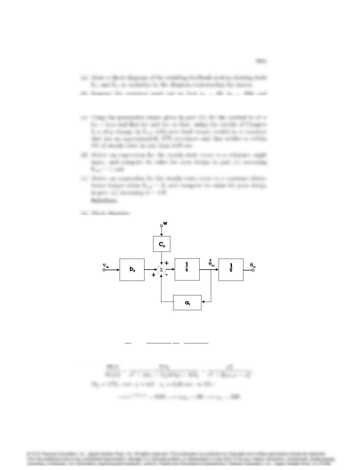
c0= 10. If there is no load torque (w= 0), what speed (in rpm)

results from va= 100 V?

Block diagram for Problem 4.26

(b) If Va=constant the system is in steady state:

_

=b0

a1

Va=200 100

65

60

2

rad:sec1

rpm = 2938 rpm:

(c)

26. We wish to design an automatic speed control for an automobile. Assume

that (1) the car has a mass mof 1000 kg, (2) the accelerator is the control

Uand supplies a force on the automobile of 10 Nper degree of accelerator

motion, and (3) air drag provides a friction force proportional to velocity

of 10 Nsec=m.

problem.

(d) Assuming that pure integral control (that is, no proportional term) is

advantageous, select the feedback gain so that the roots have critical

damping (= 1).

Solution:

E(s) = VdV=Vd

1 + kP

s+ 0:02

Vd+

1 + kP

s+ 0:02

G(s);

=(s+ 0:02)Vd0:05G

s+ 0:02 + kP

;

27. Consider the automobile speed control system depicted in Fig. 4.40.

4034 CHAPTER 4. CHAPTER 4: A FIRST ANALYSIS OF FEEDBACK

(a) Find the transfer functions from W(s)and from R(s)to Y(s).

(b) Assume that the desired speed is a constant reference r, so that

R(s) = ro=s. Assume that the road is level, so w(t) = 0. Compute

values of the gains kP,Hr, and Hyto guarantee that

lim

t!1 y(t) = ro:

Include both the open-loop (assuming Hy= 0) and feedback cases

(Hy6= 0) in your discussion.

(c) Repeat part (b) assuming that a constant grade disturbance W(s) =

wo=s is present in addition to the reference input. In particular,

find the variation in speed due to the grade change for both the feed

forward and feedback cases. Use your results to explain (1) why

feedback control is necessary and (2) how the gain kPshould be

chosen to reduce steady-state error.

(d) Assume that w(t) = 0 and that the gain Aundergoes the perturba-

tion A+A. Determine the error in speed due to the gain change

for both the feed forward and feedback cases. How should the gains

be chosen in this case to reduce the effects of A?

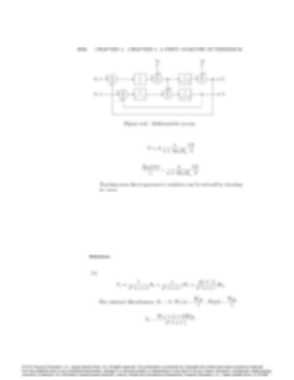
28. Consider the multivariable system shown in Fig. 4.41. Assume that the

system is stable. Find the transfer functions from each disturbance input

to each output and determine the steady-state values of y1and y2for

constant disturbances. We define a multivariable system to be Type k

with respect to polynomial inputs at wiif the steady-state value of every

output is zero for any combination of inputs of degree less than kand at

least one input is a non-zero constant for an input of degree k: What is

the system type with respect to disturbance rejection at w1? At w2?

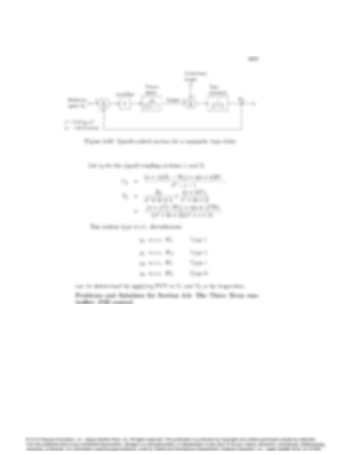
29. The transfer functions of speed control for a magnetic tape-drive system

are shown in Fig. 4.42. The speed sensor is fast enough that its dynamics

can be neglected and the diagram shows the equivalent unity feedback

system.

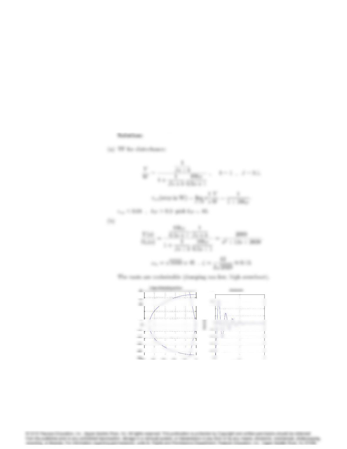
(a) Assuming the reference is zero, what is the steady-state error due to

a step disturbance torque of 1 N m? What must the amplifier gain

Kbe in order to make the steady-state error ess 0:01 rad/sec.?

(b) Plot the roots of the closed-loop system in the complex plane, and

accurately sketch the time response of the output for a step reference

input using the gain Kcomputed in part (a).

4038 CHAPTER 4. CHAPTER 4: A FIRST ANALYSIS OF FEEDBACK

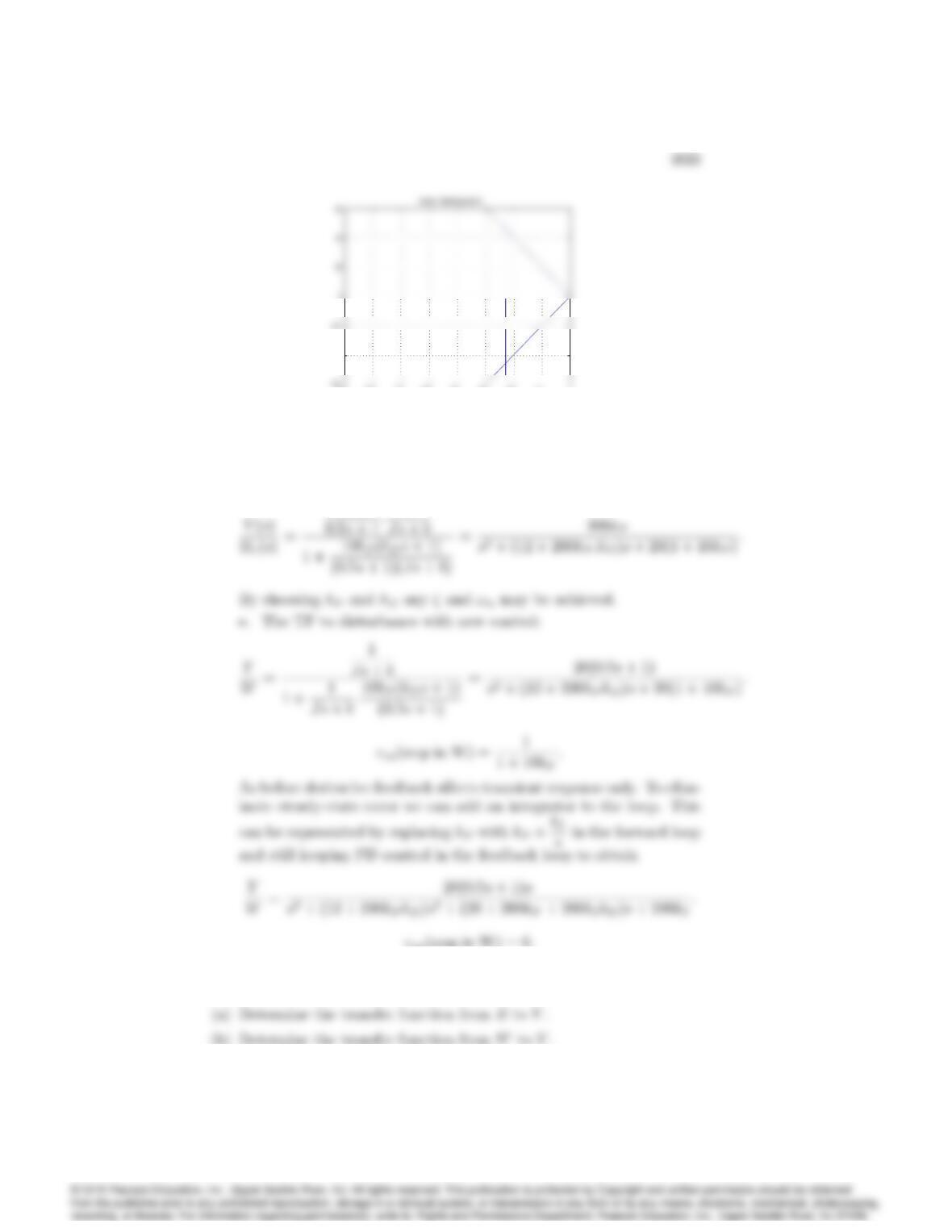
(c) Plot the region in the complex plane of acceptable closed-loop poles

corresponding to the specifications of a 1% settling time of ts

0:1sec. and an overshoot Mp5%.

(d) Give values for kPand kDfor a PD controller which will meet the

specifications.

(e) How would the disturbance-induced steady-state error change with

the new control scheme in part (d)? How could the steady-state error

to a disturbance torque be eliminated entirely?

–50 -40 –30 –20 -10 0

–40

–30

–20

–10

10

20

*

00.5 1

1.2

1.4

1.8

Ti me (sec)

(c) For ts0:1 =)46 For Mp0:05 =)0:7:

-160 -140 -120 -100 -80 –60 -40 -20 0

-40

s-plane for part(c)

(a) d. We know that larger !nand are needed. This can be achieved

by increasing kPand adding derivative feedback as in Fig. 4.8,

10kP

30. Consider the system shown in Fig. 4.43 with PI control.