4051
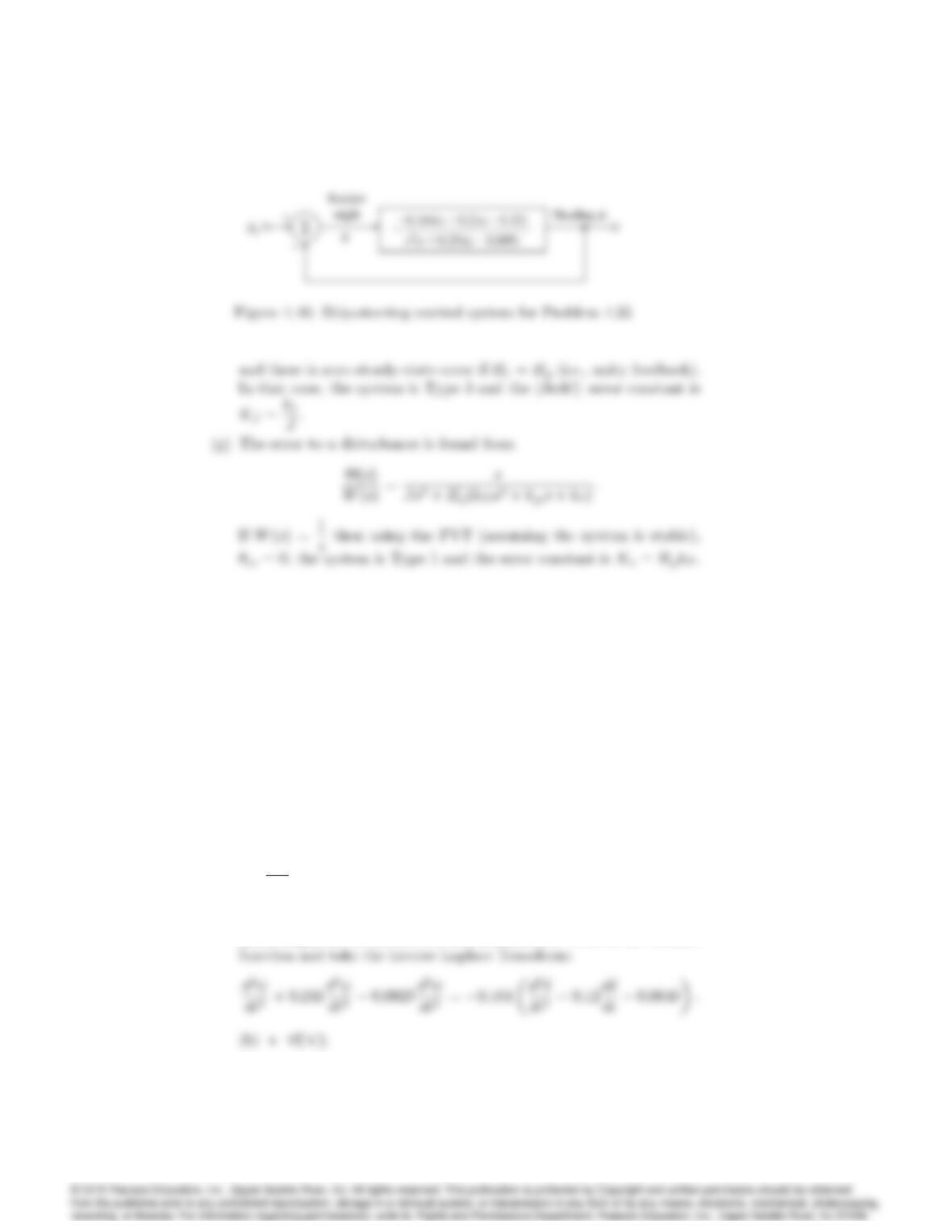
35. Automatic ship steering is particularly useful in heavy seas when it is
important to maintain the ship along an accurate path. Such a control
system for a large tanker is shown in Fig. 4.46, with the plant transfer
function relating heading changes to rudder de‡ection in radians.
(a) Write the differential equation that relates the heading angle to rud-
der angle for the ship without feedback..
(b) This control system uses simple proportional feedback with the gain
of unity. Is the closed-loop system stable as shown? (Hint: use
Routh’s criterion)
(c) Is it possible to stabilize this system by changing the proportional
gain from unity to a lower value?
(d) Use Matlab to design a dynamic controller of the form Dc(s) =
Ks+a
s+b2
so that the closed-loop system is stable and in response to
a step heading command it has zero steady-state error and less than
10% overshoot. Are these reasonable values for a large tanker?Solution:
(a) Multiply out the numerator and denominator terms in the transfer
4052 CHAPTER 4. CHAPTER 4: A FIRST ANALYSIS OF FEEDBACK
(c) The closed-loop characteristic polynomial is 1 + KpG(s) = 0 that
leads to:
(d) There are many solutions. One solution is to place the following
dynamic controller with 2 poles and 2 zeros in front of the plant:
–
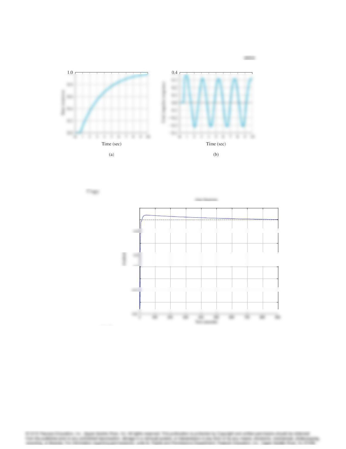
Figure 4.47: Paper-machine response data for Problem 4.36
38:pdf
–0.4
0
0.2
0.6
1
1.2
–0.4
0
0.2
0.6
1
1.2
Closed-loop step response for ship-steering, Problem 4.36
36. The unit-step response of a paper machine is shown in Fig. 4.47(a) where
the input into the system is stock ‡ow onto the wire and the output is basis
weight (thickness). The time delay and slope of the transient response may
be determined from the figure.
(a) Find the proportional, PI, and PID-controller parameters using the
4054 CHAPTER 4. CHAPTER 4: A FIRST ANALYSIS OF FEEDBACK
Zeigler–Nichols transient-response method.
(b) Using proportional feedback control, control designers have obtained
a closed-loop system with the unit impulse response shown in Fig. 4.47(b).
When the gain Ku= 8:556, the system is on the verge of instabil-
ity. Determine the proportional-, PI-, and PID-controller parameters
according to the Zeigler–Nichols ultimate sensitivity method.
Solution:
(a) From step response: L=d‘0:65 sec
From Table 4.1:
(b) From the impulse response: Pu‘2:33 sec. and from Table 4.2:
37. A paper machine has the transfer function
G(s) = e2s
3s+ 1;
where the input is stock ‡ow onto the wire and the output is basis weight
or thickness.
(a) Find the PID-controller parameters using the Zeigler–Nichols tuning
rules.
(b) The system becomes marginally stable for a proportional gain of
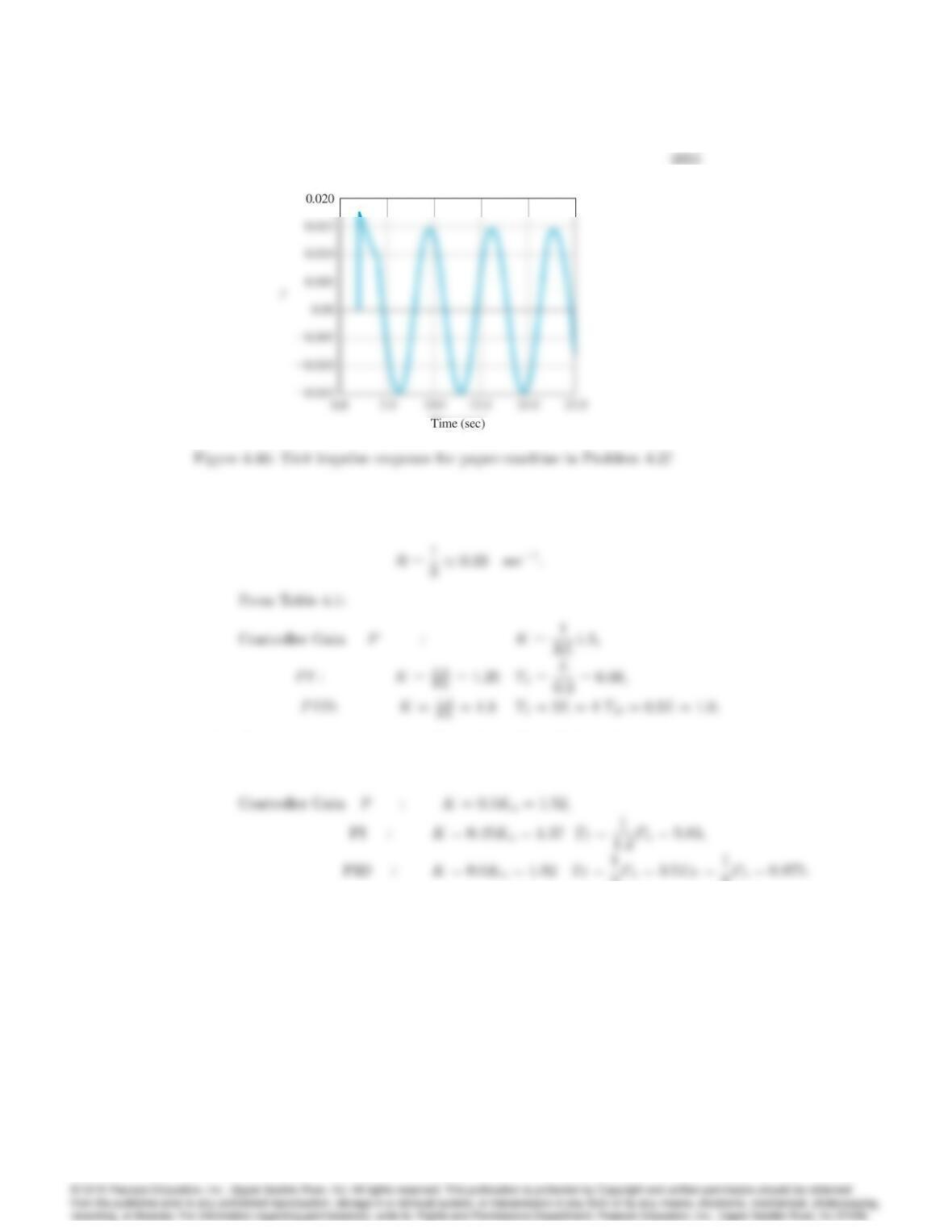
Ku= 3:044 as shown by the unit impulse response in Fig. 4.48.
Find the optimal PID-controller parameters according to the Zeigler–
Nichols tuning rules.
Solution:
(a) From the transfer function: L=d‘2sec
(b) From the impulse response: Pu‘7sec From Table 4.2:
2Pu= 3:5TD=1
8Pu= 0:875.
Problem and Solution for Section 4.4: Feedforward Control by
Plant Model Inversion
38. Consider the DC motor speed control system shown in Fig. 4.49 with
proportional control. (a) Add feedforward control to eliminate the steady-
state tracking error for a step reference input. (b) Also add feedforward
control to eliminate the effect of a constant output disturbance signal on
the output of the system.
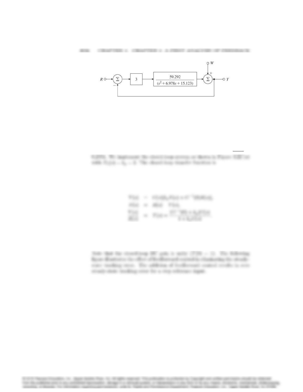
Figure 4.49: Block diagram for Problem 4.38
Solution: (a) In this case the plant inverse DC gain is G1(0) = 15:123
59:292 =
0 1 2 3 4 5
0
0.5
1.5
Time (sec)
0 1 2 3 4 5
0
0.5
1.5
Time (sec)
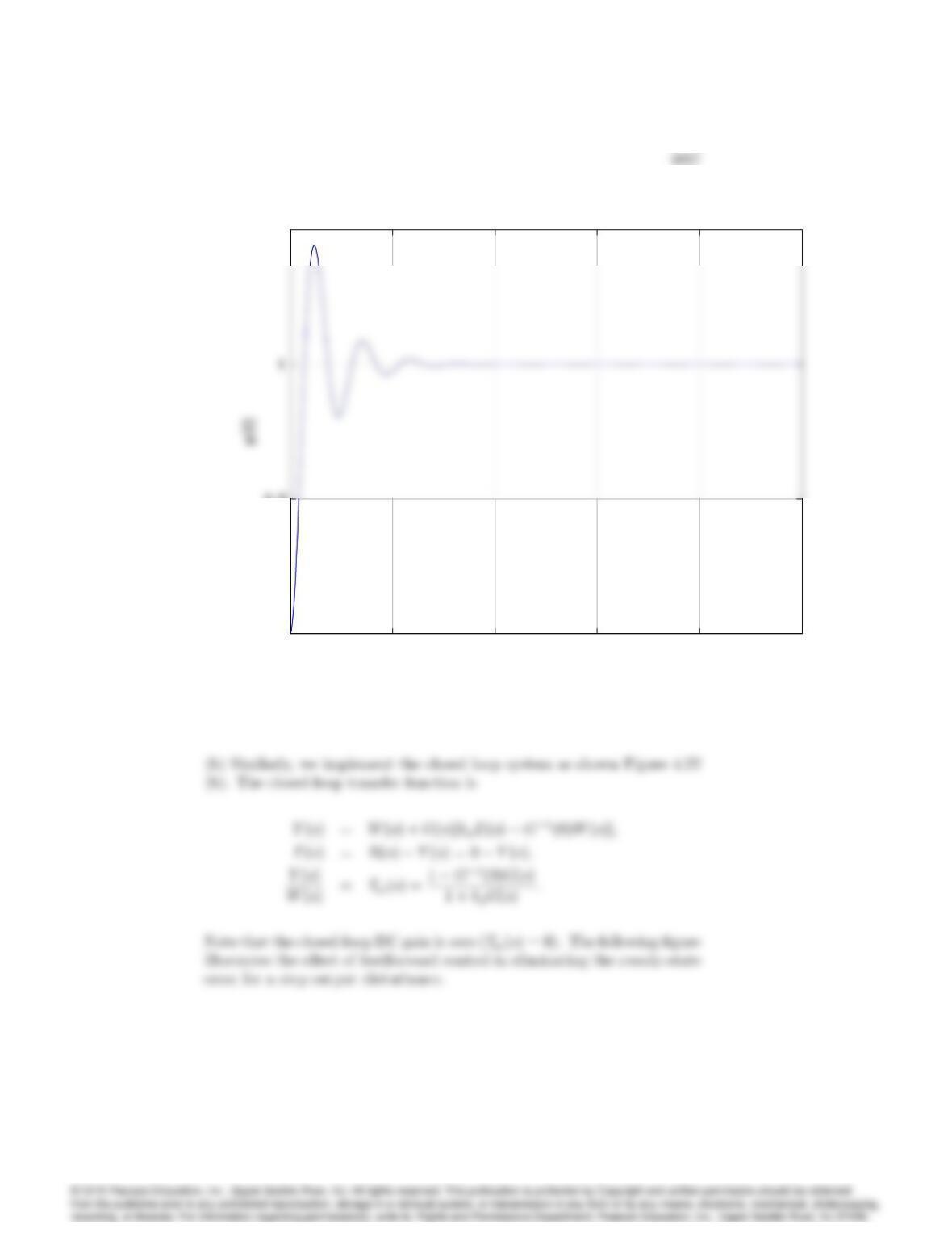
Tracking response with feedforward
4058 CHAPTER 4. CHAPTER 4: A FIRST ANALYSIS OF FEEDBACK
0 1 2 3 4 5
–0.5
0.5
Time (sec)
0 1 2 3 4 5
–0.5
0.5
Time (sec)
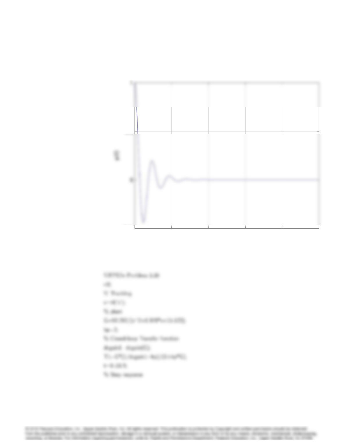
Disturbance rejection response with feedforward
MATLAB code:
4059
y1=step(T1,t);
Problems and Solutions for Section 4.5: Introduction to Digital
Control
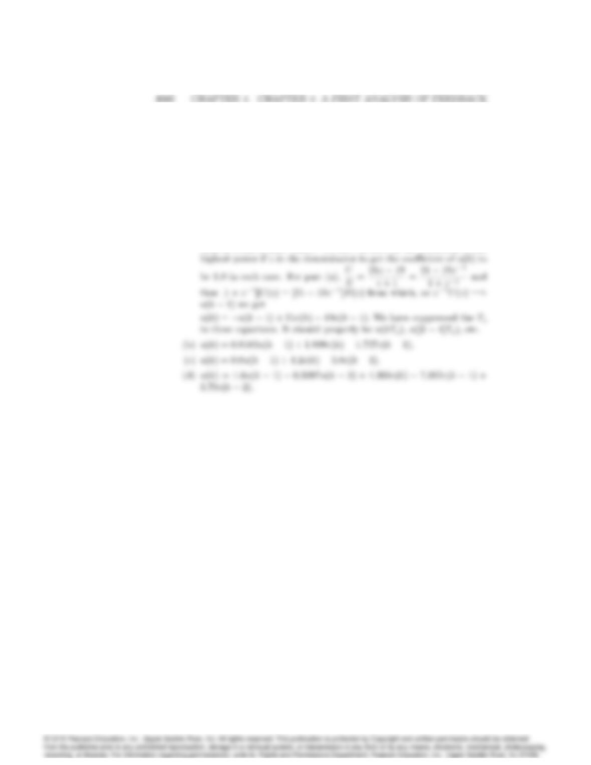
39. Compute the discrete equivalents for the following possible controllers us-
ing the trapezoid rule of Eq. (w14) in Appendix W4.5. Let Ts= 0:05 sec
in each case.
(a) Dc1(s) = (s+ 2)=2,
(b) Dc2(s) = 2s+ 2
s+ 4,
(c) Dc3(s) = 5(s+ 2)
s+ 10 ,
(d) Dc4(s) = 5 (s+ 2)(s+ 0:1)
(s+ 10)(s+ 0:01):
Solution:
40. Give the difference equations corresponding to the discrete controllers
found in Problem 4.39 respectively
(a) part 1,
(b) part 2,
(c) part 3,
(d) part 4.
Solution:
(a) Reduce the ztransforms to be in terms of z1if you want the equa-
tions in terms of past values. We have divided by the coefficient of the