3040 CHAPTER 3. DYNAMIC RESPONSE
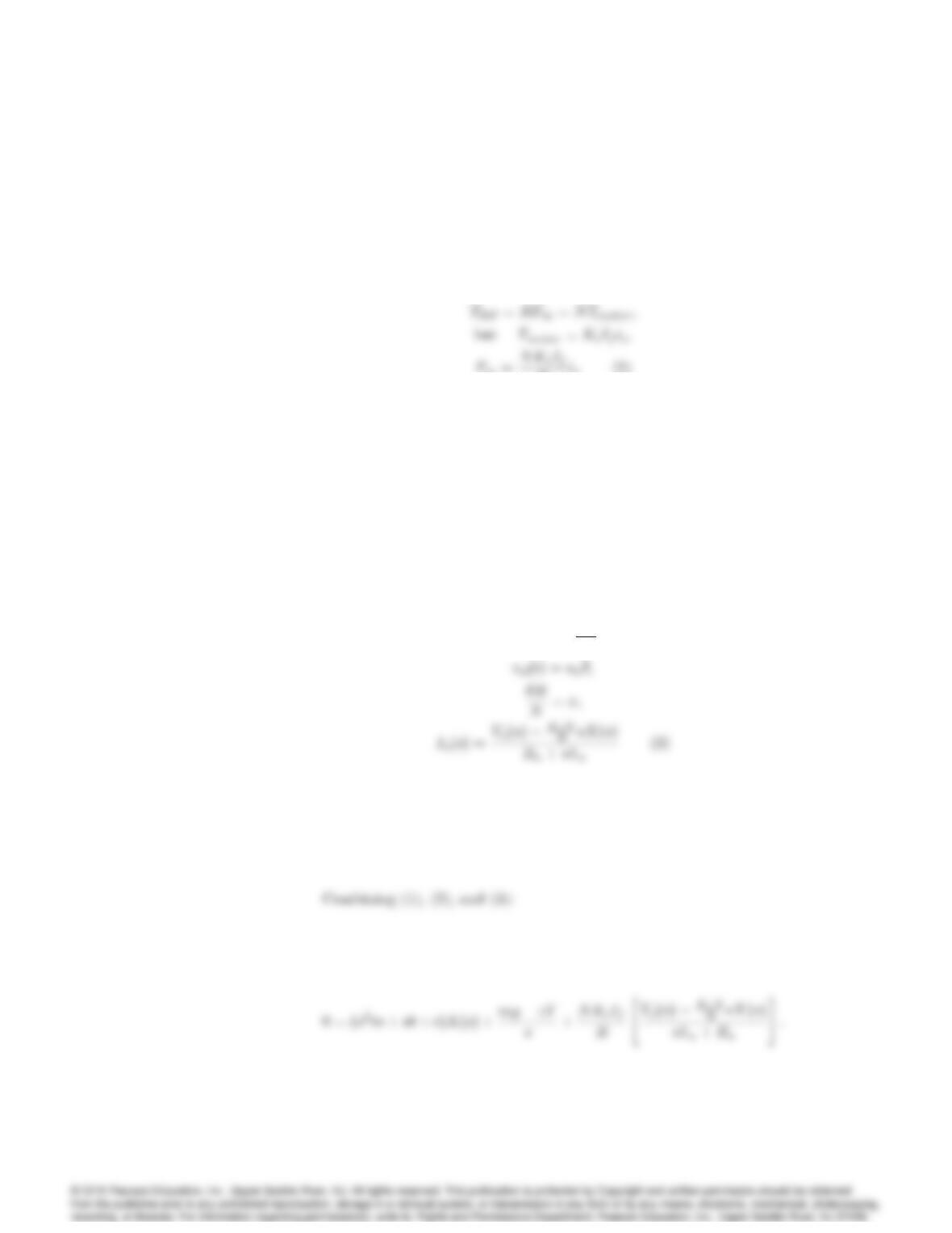
Torque in rack and pinion:
Rio(2)
DC motor circuit analysis:
vs(t) = Raio+La
dio
dt +va(t);
3041
Problems and Solutions for Section 3.2: Sys–
tem Modeling Diagrams
19. Consider the block diagram shown in Fig. 3.49. Note that aiand biare
constants. Compute the transfer function for this system. This spe-
cial structure is called the “control canonical form” and will be discussed
further in Chapter 7.
Solution:
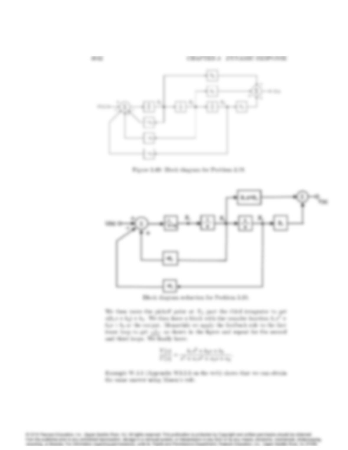
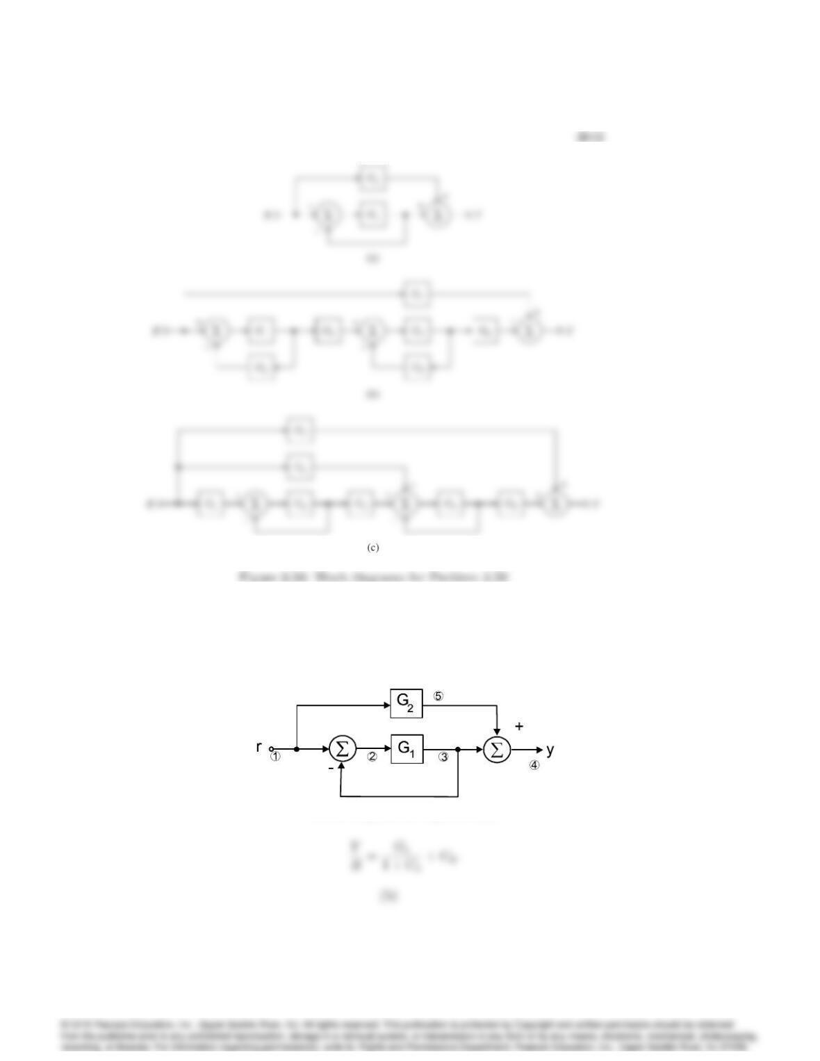
20. Find the transfer functions for the block diagrams in Fig. 3.50.
Solution:
(a)
Block diagram for Fig. 3.50 (a)
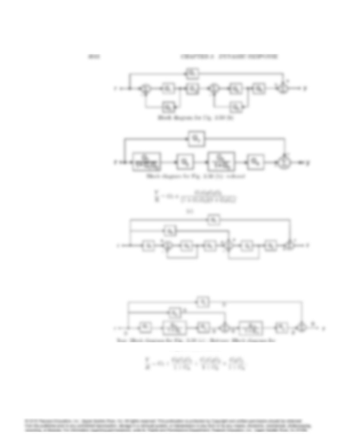
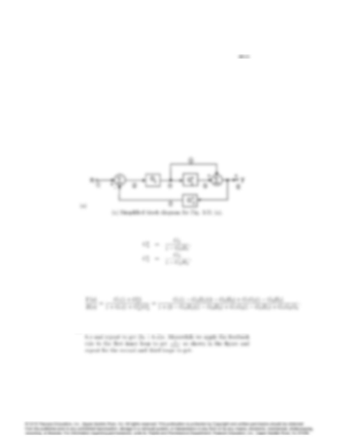
Fig 3.50 (c) reduced.
21. Find the transfer functions for the block diagrams in Fig. 3.51, using the
ideas of block diagram simplification. The special; structure in Fig. 3.51
(b) is called the “observer canonical form” and will be discussed in Chap-
ter 7.
Solution:
Part (a): Transfer functions found using the ideas of Figs. 3.9 and 3.10:
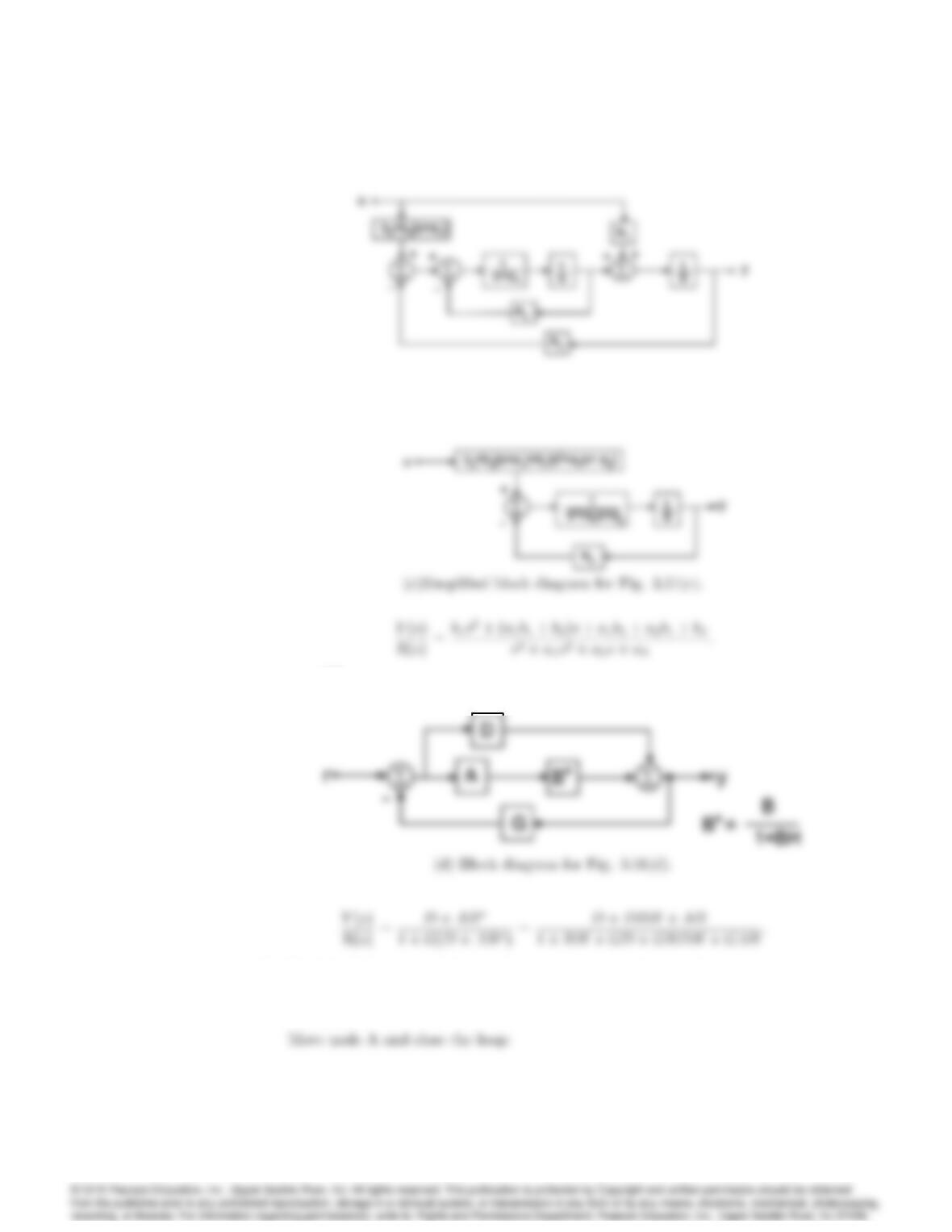
(b) We move the summer on the right hand side past the integrator to get
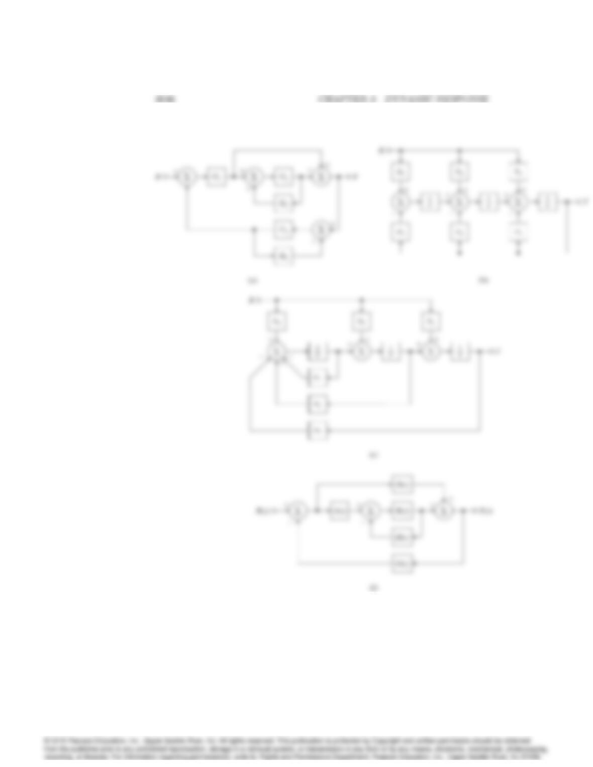
Figure 3.51: Block diagrams for Problem 3.21
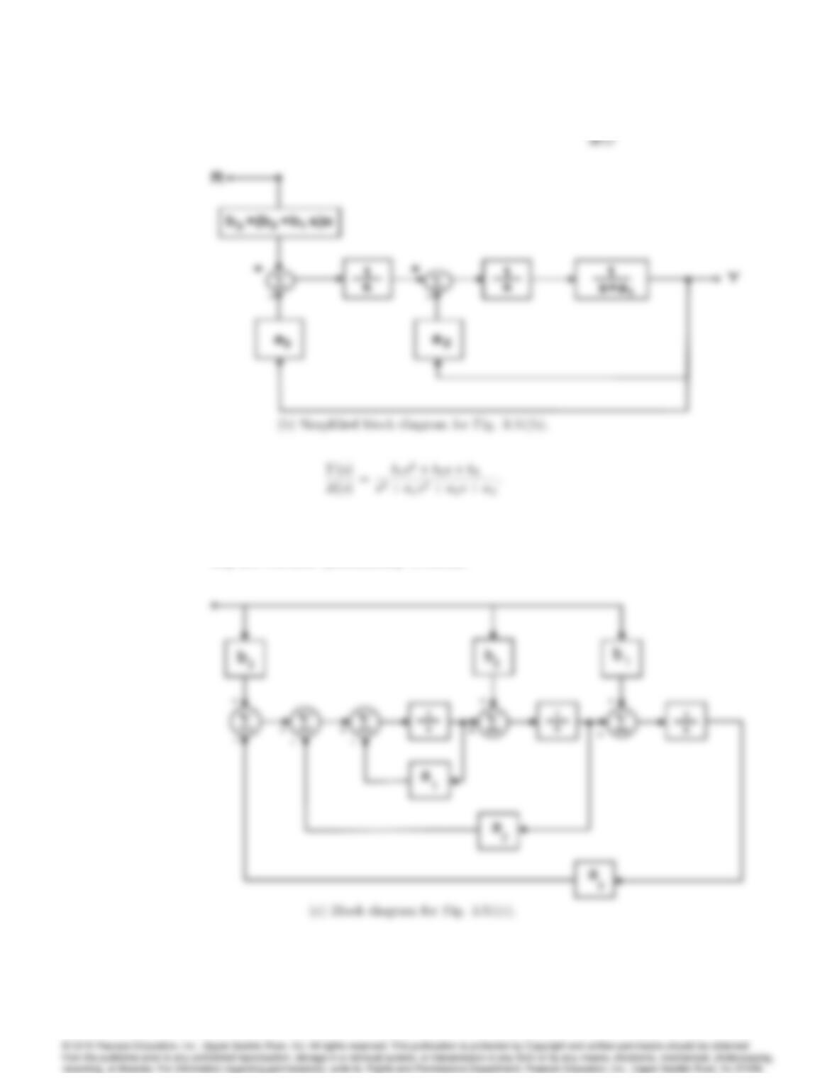
(c) Applying block diagram reduction: reduce the innermost loop, shift
b2to the b3node by mutiplying by (s+a1), reduce the next innermost
loop and continue systematically to obtain:
3048 CHAPTER 3. DYNAMIC RESPONSE
(d)
22. Use block-diagram algebra to determine the transfer function between
R(s)and Y(s)in Fig. 3.52.
Solution:
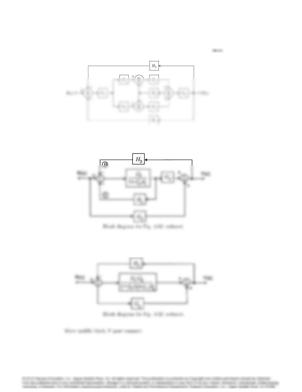
Figure 3.52: Block diagram for Problem 3.22
Add signal B, close loop and multiply before signal C:
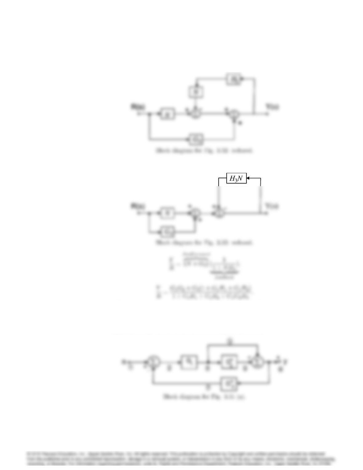
3050 CHAPTER 3. DYNAMIC RESPONSE
Now reverse order of summers and close each block separately:
23. NFind the transfer functions for the block diagrams in Fig. 3.51, using
Mason’s rule.
Solution: Transfer functions are found using Mason’s rule,
3051
(a) Mason’s rule for Fig. 3.51(a):
Forward Path Gains
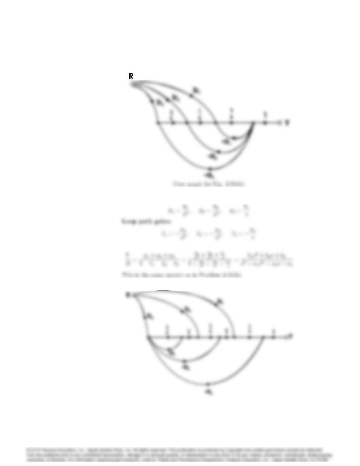
(b) Mason’s rule for Fig. 3.51(b):
3052 CHAPTER 3. DYNAMIC RESPONSE
Forward path gains:
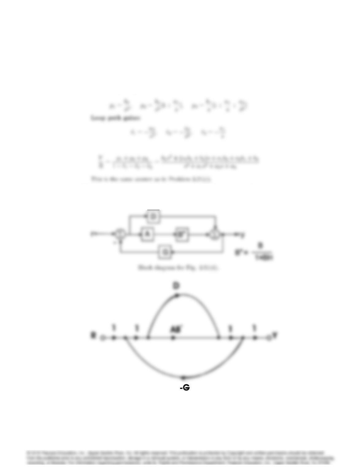
(c) Mason’s Rule for Fig. 3.51(c):
3053
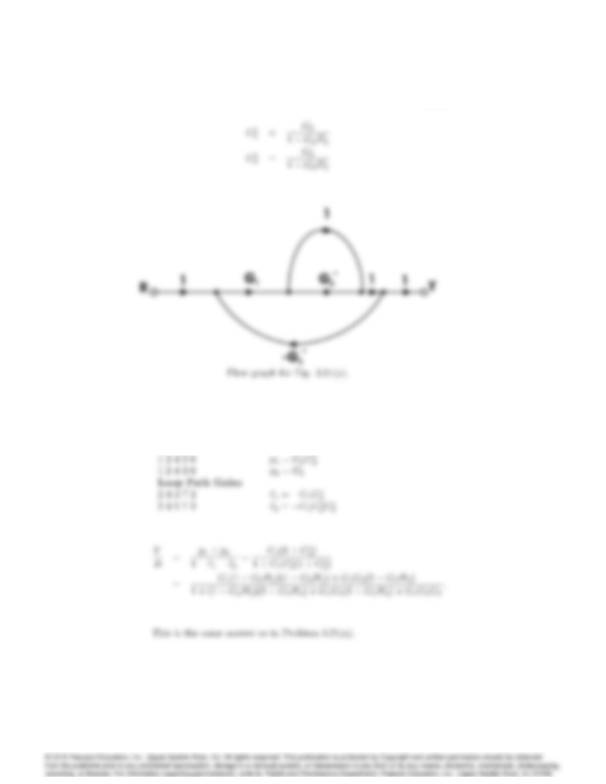
Flow graph for Fig. 3.51(c).
Forward path gains:
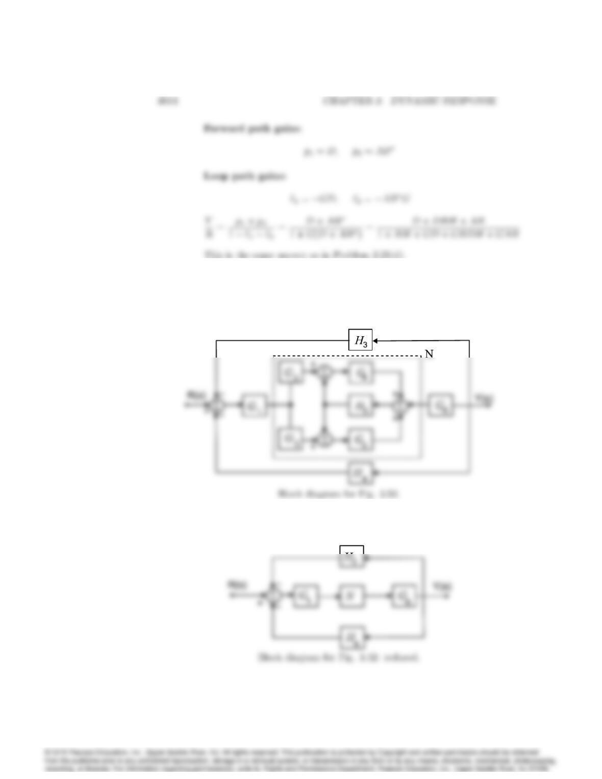
(d) Mason’s rule for Fig. 3.51(d): The system is tightly connected, easy
to apply Mason’s rule.
Flow graph for Fig. 3.51(d).
24. NUse block-diagram algebra or Mason’s rule to determine the transfer
function between R(s)and Y(s)in Fig. 3.52.
Solution:
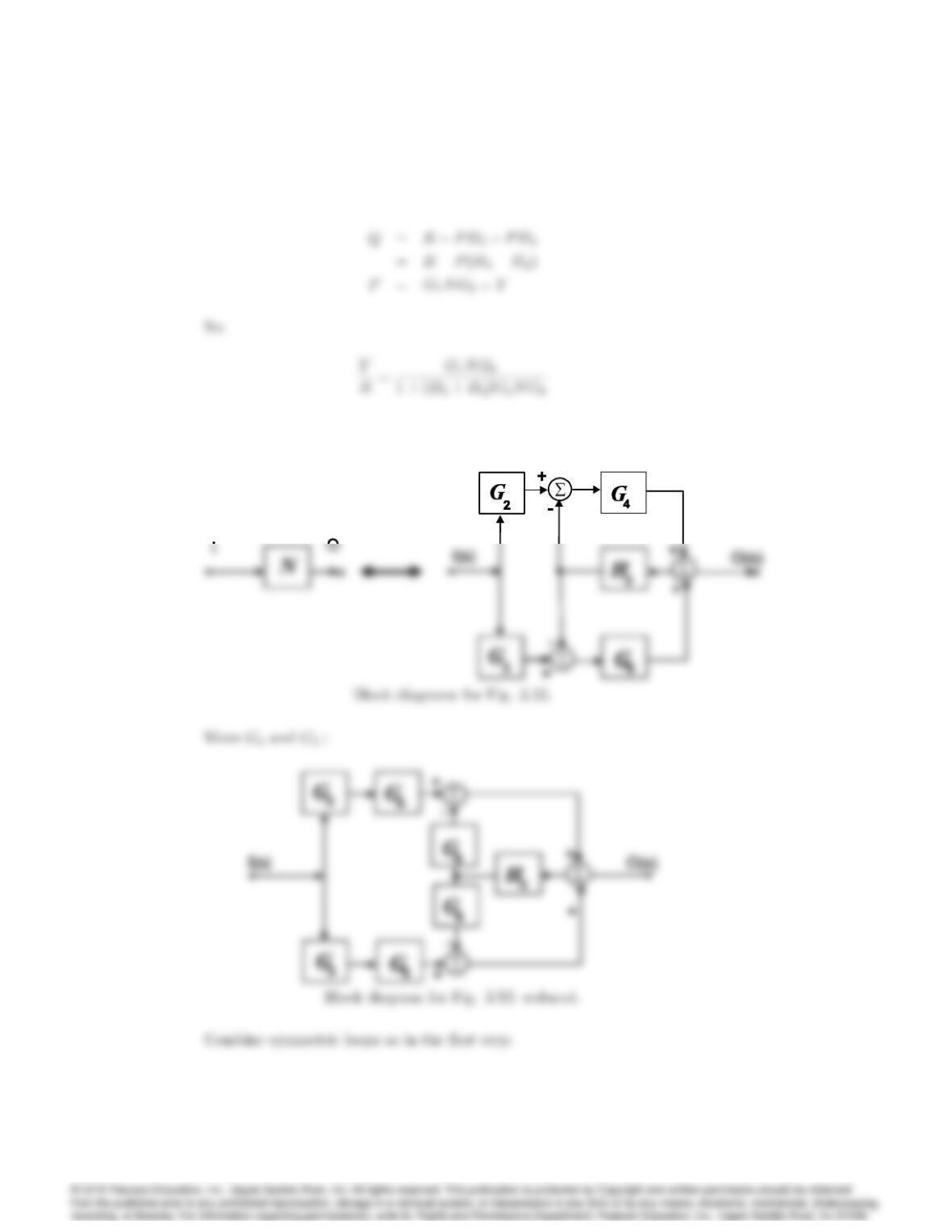
Block diagram algebra:
3055
Now, what is N?
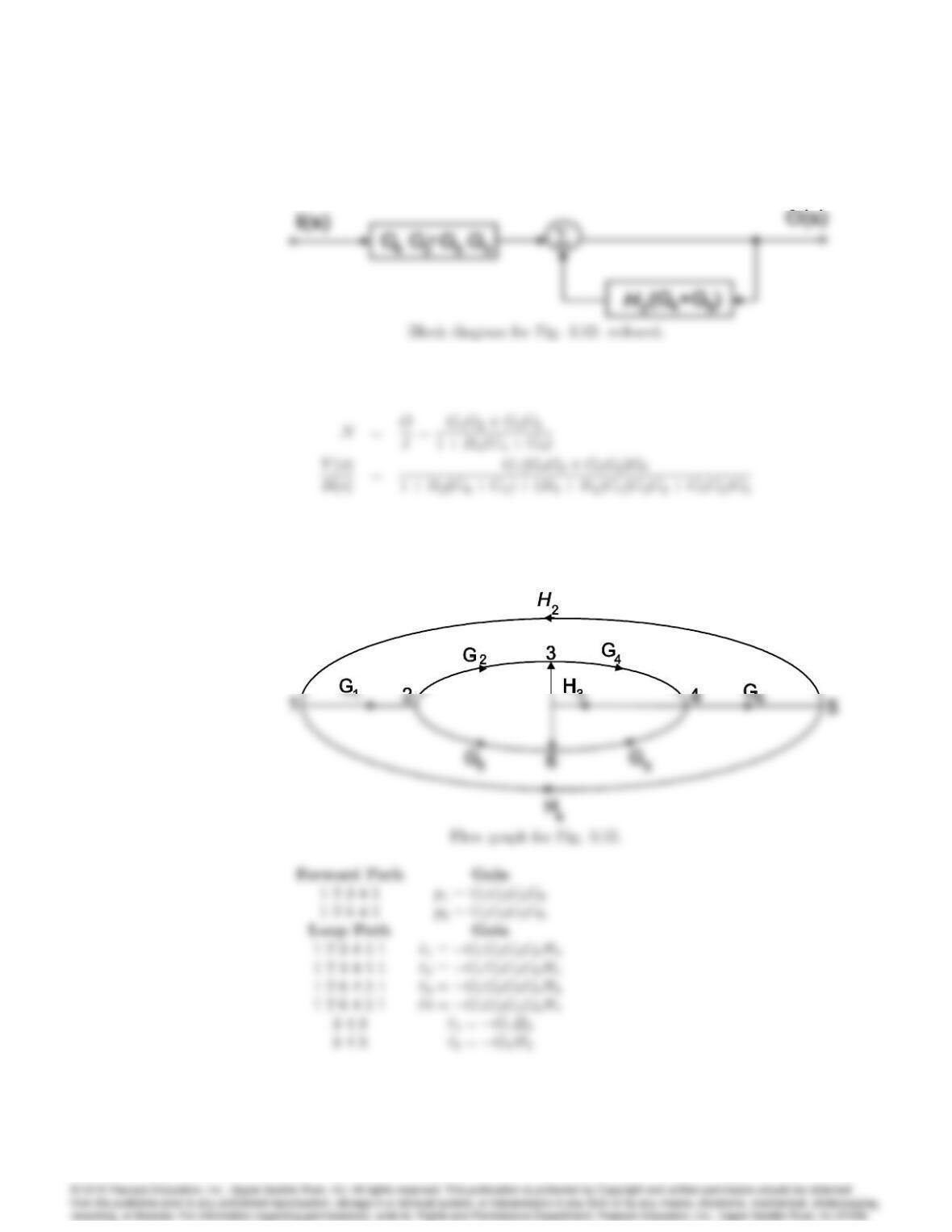
3056 CHAPTER 3. DYNAMIC RESPONSE
Which is:
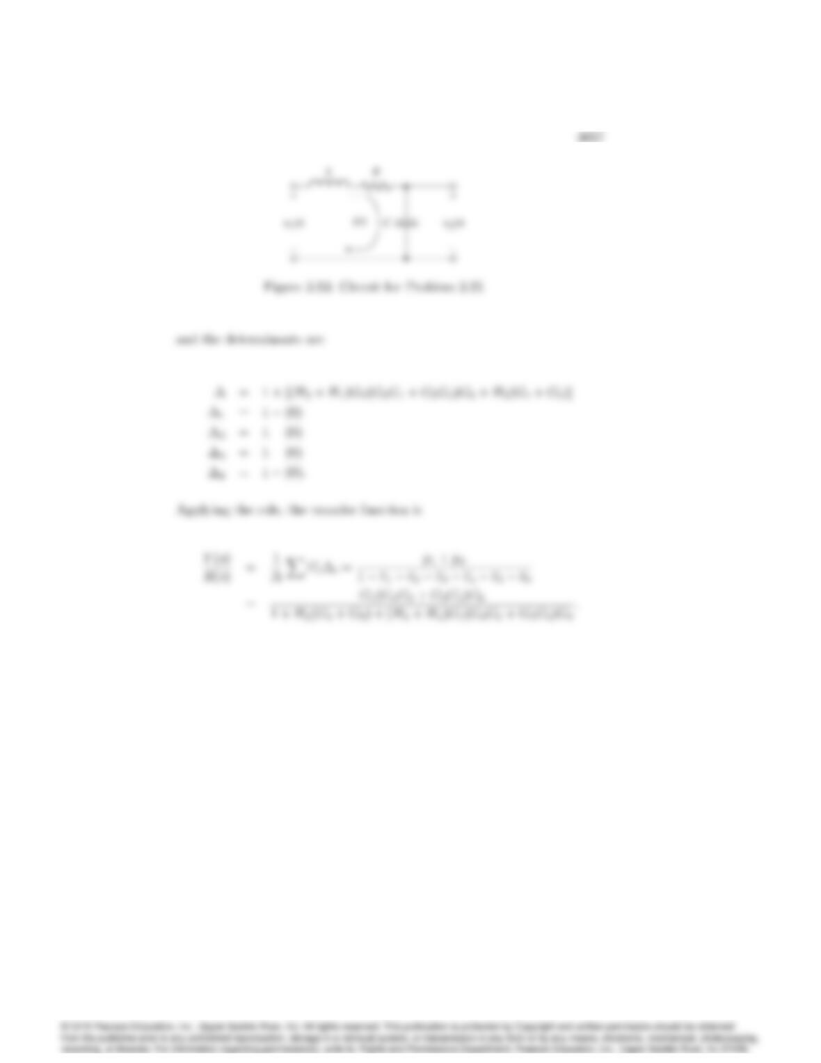
Mason’s Rule:
The signal ‡ow graph is:
Problems and Solutions for Section 3.3: E¤ect
of Pole Locations
25. For the electric circuit shown in Fig. 3.53, find the following:
(a) The time-domain equation relating i(t) and v1(t);
(b) The time-domain equation relating i(t) and v2(t);
(c) Assuming all initial conditions are zero, the transfer function V2(s)=V1(s)
and the damping ratio and undamped natural frequency !nof the
system;
(d) The values of R that will result in v2(t)having an overshoot of no
more than 25%, assuming v1(t)is a unit step, L = 10 mH, and
C= 4 F.
Solution:
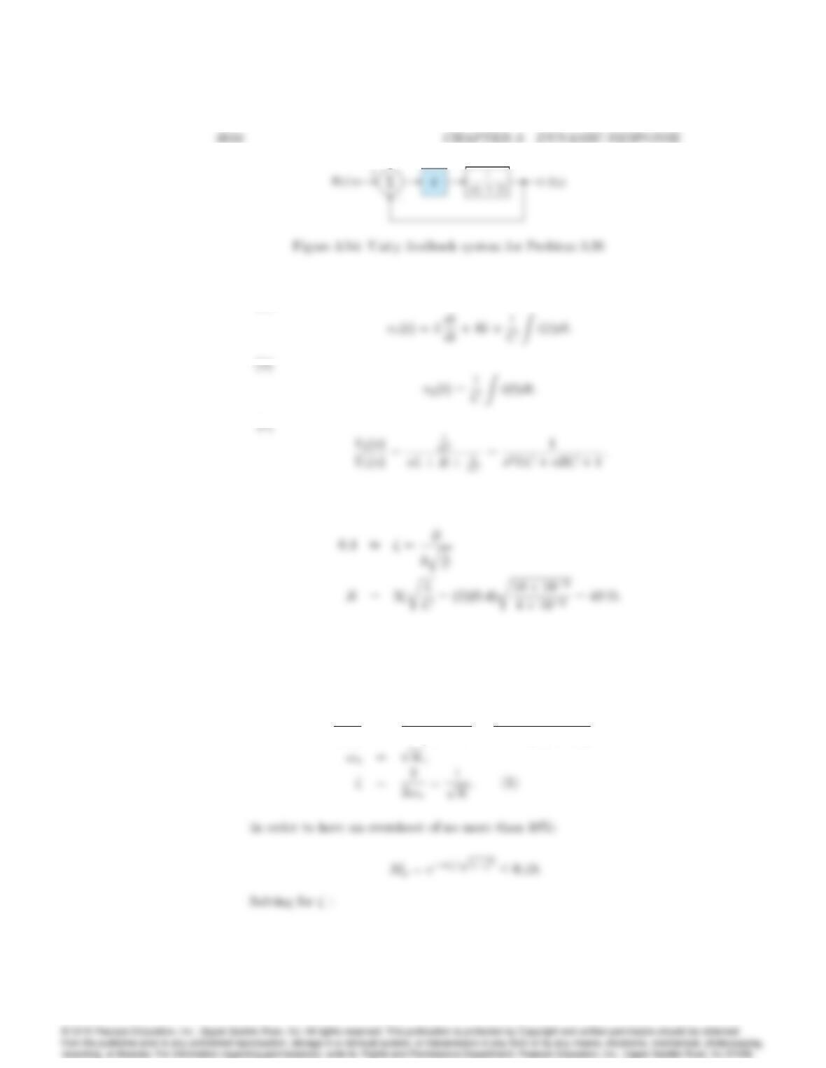
(a)
(d) For 25% overshoot t0:4,
26. For the unity feedback system shown in Fig. 3.54, specify the gain Kof
the proportional controller so that the output y(t)has an overshoot of no
more than 10% in response to a unit step.
Solution:
Y(s)
R(s)=K
s2+ 2s+K=!2
n
s2+ 2!ns+!2
n
;
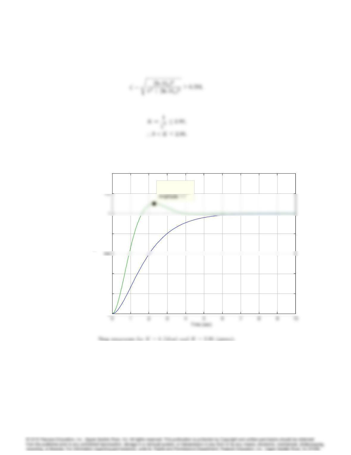
3059
Using (1) and the solution for :
0.2
0.4
0.8
1.4
Step Response
Amplitude
0.2
0.4
0.8
1.4
System: sys
Time ( sec): 2.29
27. For the unity feedback system shown in Fig. 3.55, specify the gain and
pole location of the compensator so that the overall closed-loop response
to a unit-step input has an overshoot of no more than 25%, and a 1%
settling time of no more than 0.1 sec. Verify your design using Matlab.
Solution: