Operating Systems Chapter 2 Homework The key is to draw the Free Body Diagram

2000

Solutions Manual: Chapter 2

7th Edition

Feedback Control of Dynamic

Systems

Gene F. Franklin

.J. David Powell

.Abbas Emami-Naeini

Assisted by:

H. K. Aghajan

H. Al-Rahmani

P. Coulot

P. Dankoski

S. Everett

R. Fuller

T. Iwata

V. Jones

F. Safai

L. Kobayashi

H-T. Lee

E. Thuriyasena

M. Matsuoka

Chapter 2

Dynamic Models

Problems and Solutions for Section 2.1

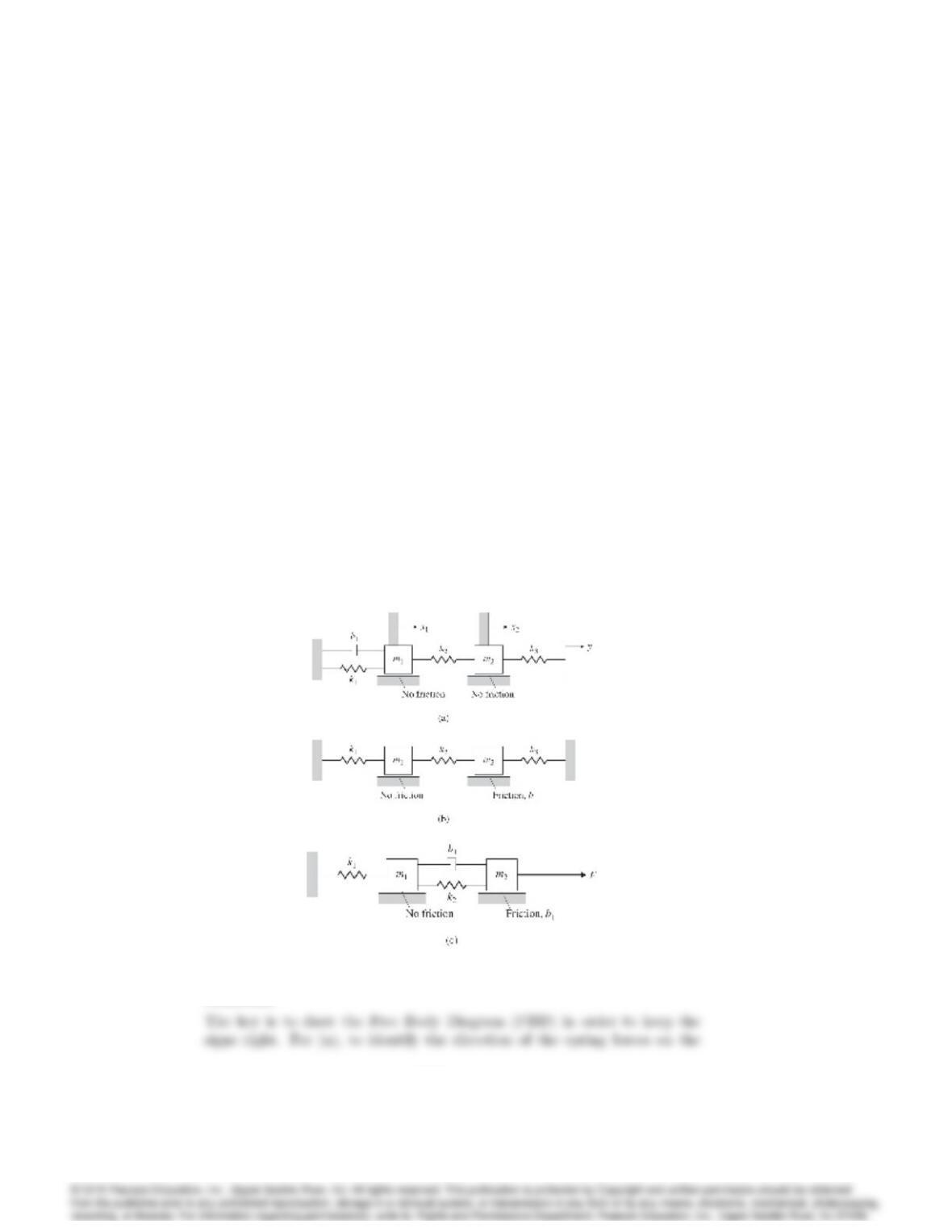
1. Write the differential equations for the mechanical systems shown in Fig. 2.41.

For (a) and (b), state whether you think the system will eventually de-

cay so that it has no motion at all, given that there are non-zero initial

conditions for both masses, and give a reason for your answer.

Fig. 2.41 Mechanical systems

Solution:

2001

2002 CHAPTER 2. DYNAMIC MODELS

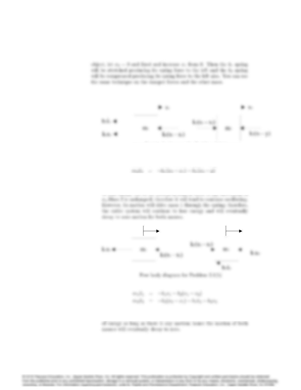
(a)

Free body diagram for Problem 2.1(a)

m1•x1=k1x1b1_x1k2(x1x2)

There is friction affecting the motion of mass 1 which will continue

to take energy out of the system as long as there is any movement of

x1x2

x2

Again, there is friction on mass 2 so there will continue to be a loss

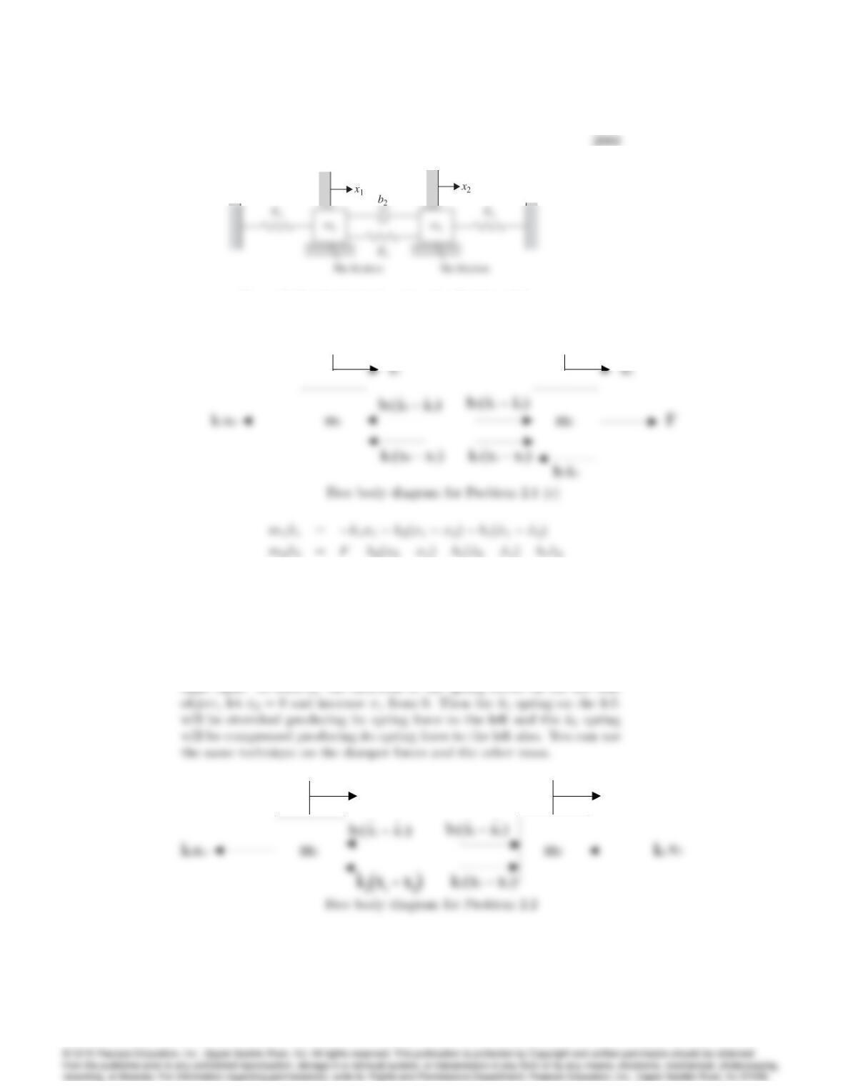
Figure 2.42: Mechanical system for Problem 2.2

2. Write the differential equations for the mechanical systems shown in Fig. 2.42.

State whether you think the system will eventually decay so that it has

no motion at all, given that there are non-zero initial conditions for both

masses, and give a reason for your answer.

Solution:

The key is to draw the Free Body Diagram (FBD) in order to keep the

signs right. To identify the direction of the spring forces on the left side

x1x2

2004 CHAPTER 2. DYNAMIC MODELS

Then the forces are summed on each mass, resulting in

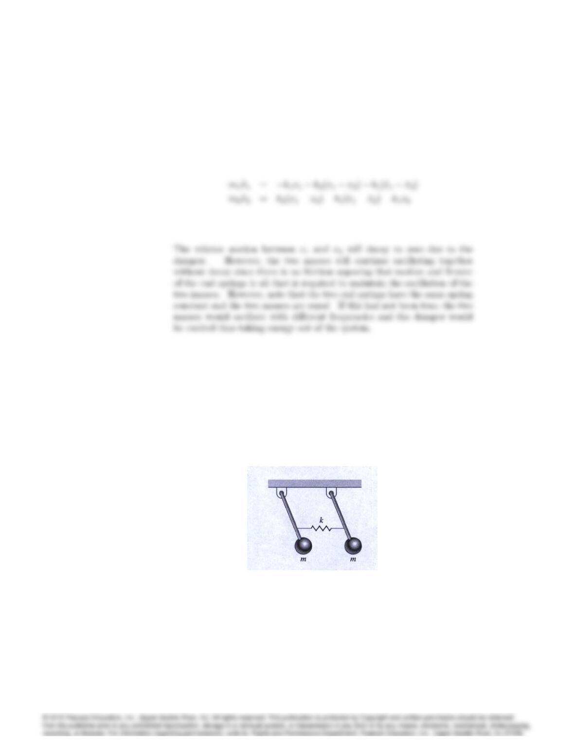
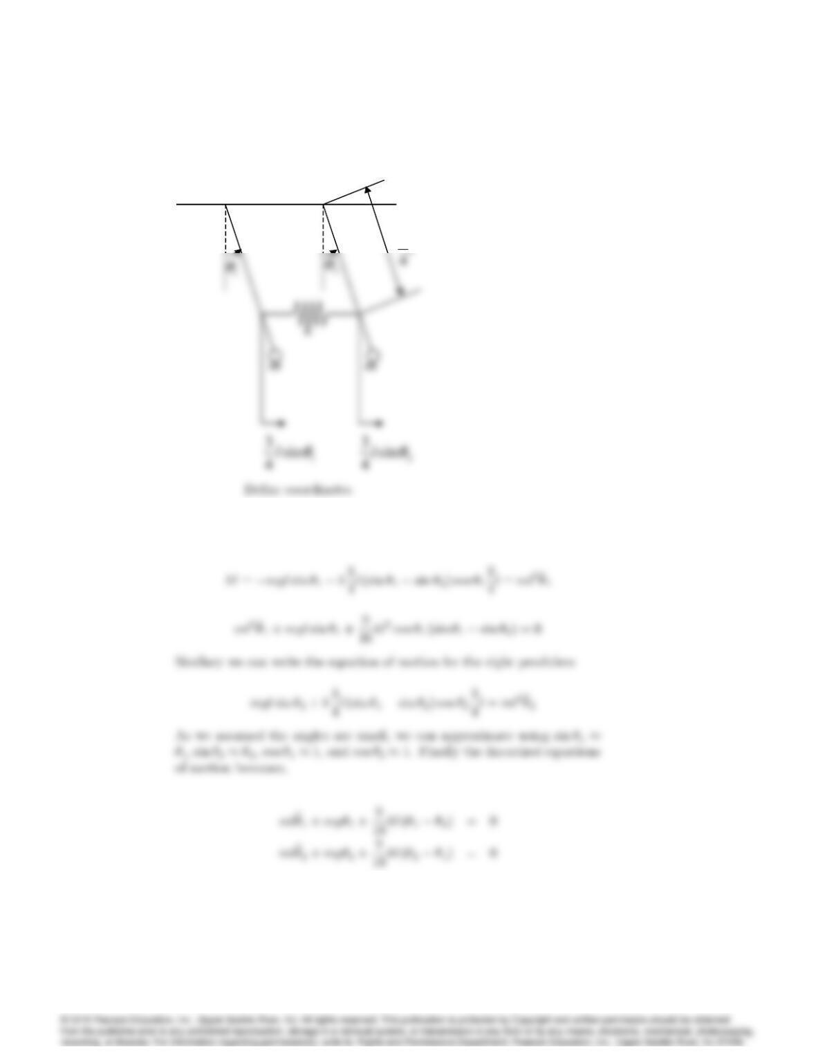
3. Write the equations of motion for the double-pendulum system shown in

Fig. 2.43. Assume the displacement angles of the pendulums are small

enough to ensure that the spring is always horizontal. The pendulum

rods are taken to be massless, of length l, and the springs are attached

3/4 of the way down.

Figure 2.43: Double pendulum

Solution:

2005

3

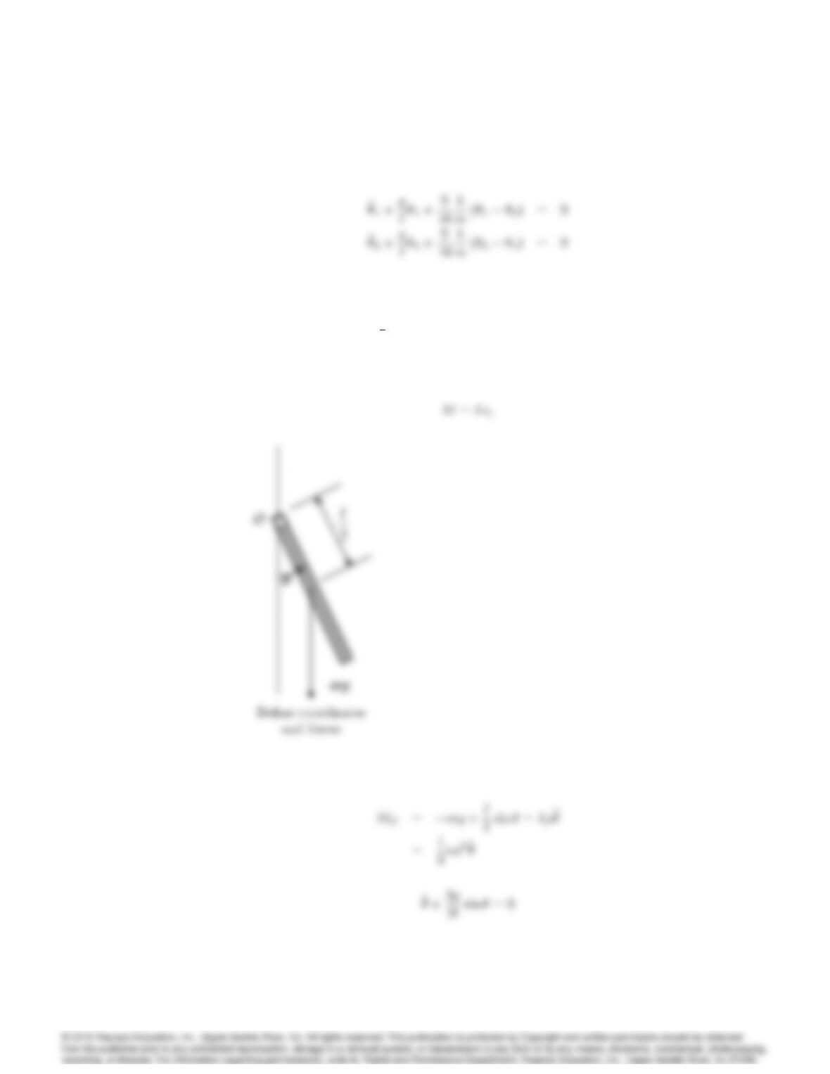
If we write the moment equilibrium about the pivot point of the left pen-

dulem from the free body diagram,

Or

2006 CHAPTER 2. DYNAMIC MODELS

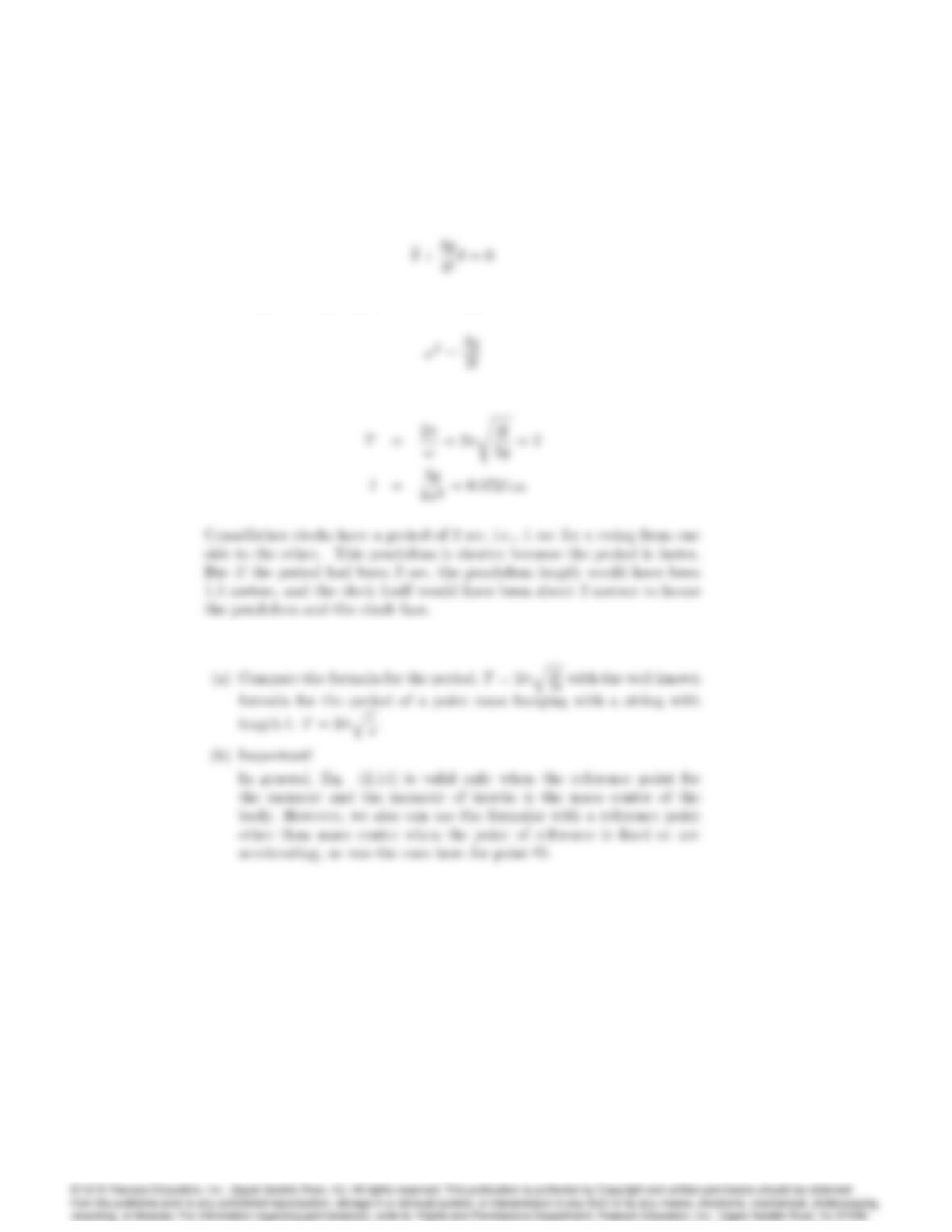
4. Write the equations of motion of a pendulum consisting of a thin, 2-kg

stick of length lsuspended from a pivot. How long should the rod be in

order for the period to be exactly 1 sec? (The inertia Iof a thin stick

about an endpoint is 1

3ml2. Assume is small enough that sin 

=.)

Solution:

Let’s use Eq. (2.14)

Moment about point O.

2007

As we assumed is small,

The frequency only depends on the length of the rod

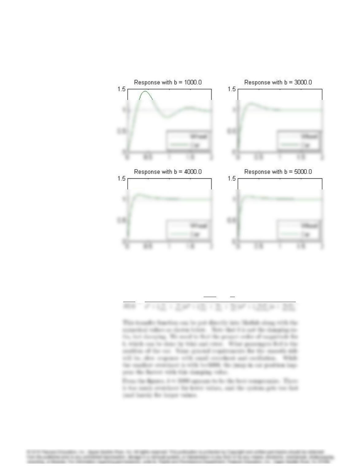
5. For the car suspension discussed in Example 2.2, plot the position of the

car and the wheel after the car hits a “unit bump” (i.e., ris a unit step)

using Matlab. Assume that m1= 10 kg,m2= 250 kg,kw= 500;000 N=m,

ks= 10;000 N=m. Find the value of bthat you would prefer if you were

a passenger in the car.

Solution:

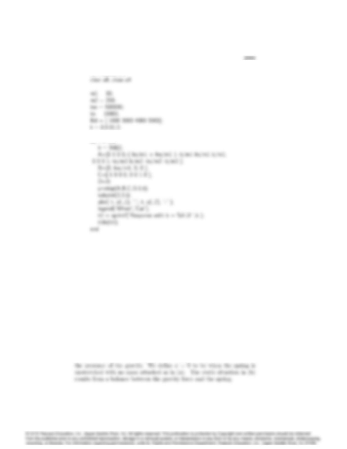
The transfer function of the suspension was given in the example in Eq.

(2.12) to be:

2008 CHAPTER 2. DYNAMIC MODELS

(a)

Y(s)

kwb

m1m2(s+ks

b)

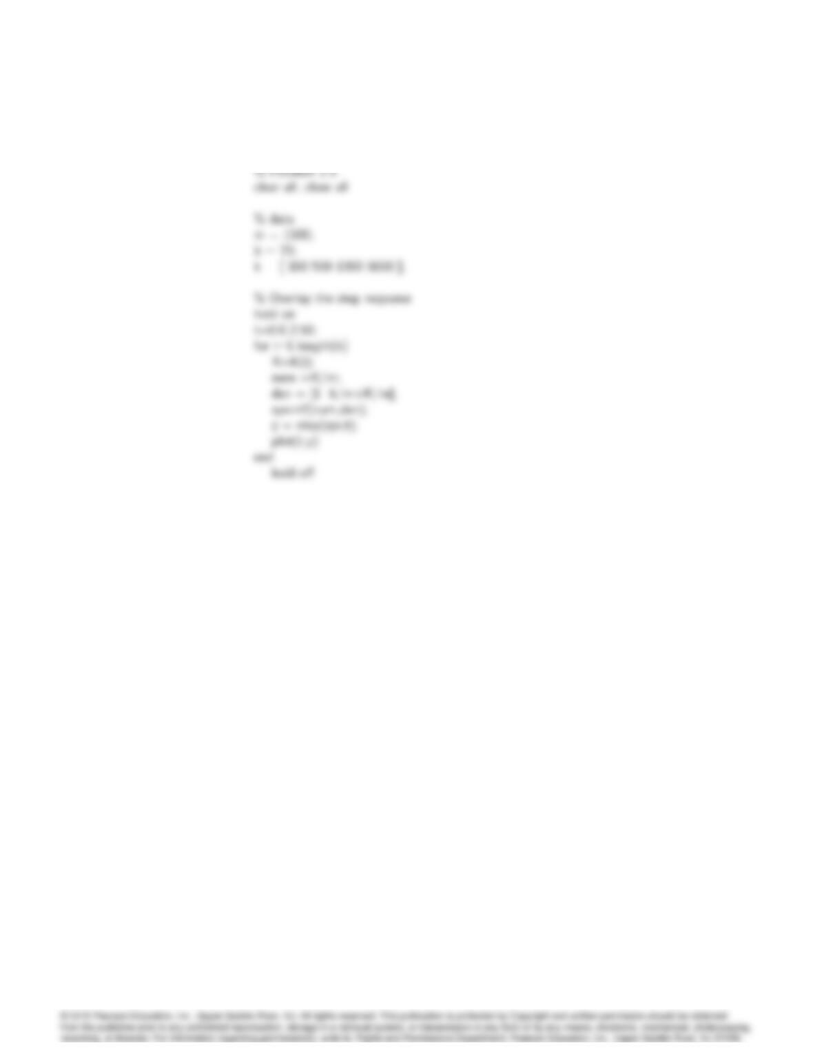
% Problem 2.5

6. Write the equations of motion for a body of mass Msuspended from a

fixed point by a spring with a constant k. Carefully define where the

body’s displacement is zero.

Solution:

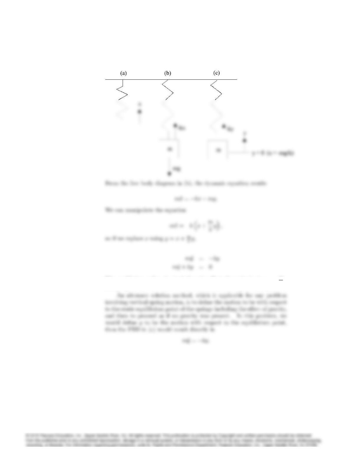
Some care needs to be taken when the spring is suspended vertically in

2010 CHAPTER 2. DYNAMIC MODELS

The equilibrium value of xincluding the effect of gravity is at x=m

kg

and yrepresents the motion of the mass about that equilibrium point.

7. Automobile manufacturers are contemplating building active suspension

systems. The simplest change is to make shock absorbers with a change-

able damping, b(u1):It is also possible to make a device to be placed in

parallel with the springs that has the ability to supply an equal force, u2;

in opposite directions on the wheel axle and the car body.

2011

(a) Modify the equations of motion in Example 2.2 to include such con-

trol inputs.

(b) Is the resulting system linear?

(c) Is it possible to use the forcer, u2;to completely replace the springs

and shock absorber? Is this a good idea?

Solution:

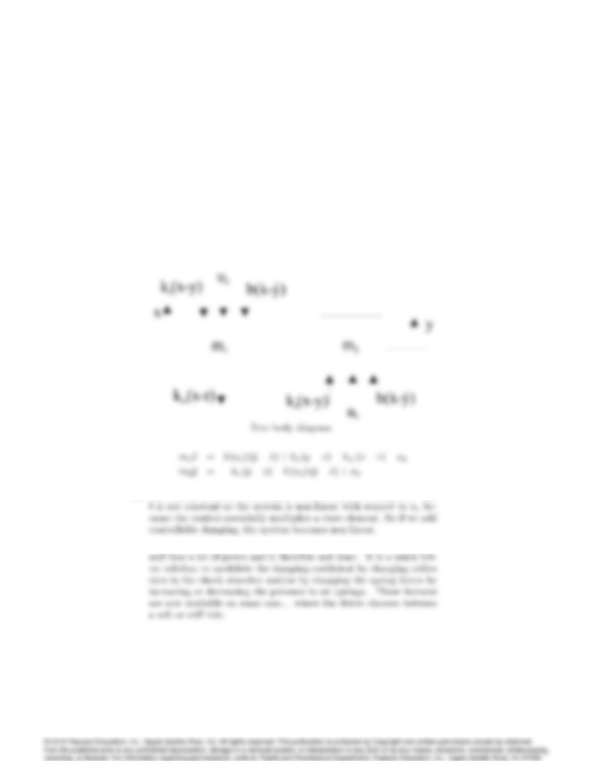
(a) The FBD shows the addition of the variable force, u2;and shows b

as in the FBD of Fig. 2.5, however, here bis a function of the control

variable, u1:The forces below are drawn in the direction that would

result from a positive displacement of x.

(b) The system is linear with respect to u2because it is additive. But

(c) It is technically possible. However, it would take very high forces

8. In many mechanical positioning systems there is ‡exibility between one

part of the system and another. An example is shown in Figure 2.6

2012 CHAPTER 2. DYNAMIC MODELS

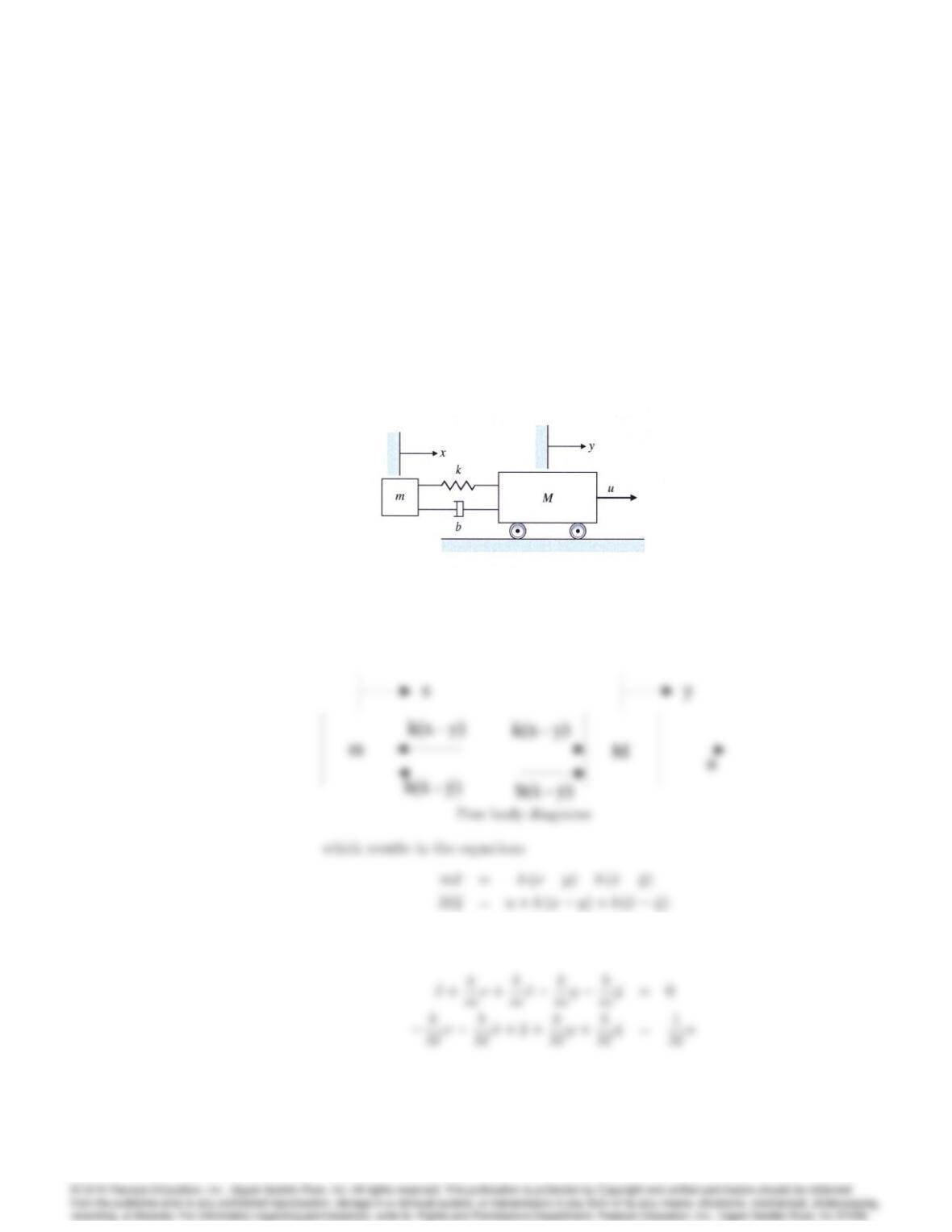
where there is ‡exibility of the solar panels. Figure 2.44 depicts such a

situation, where a force uis applied to the mass Mand another mass

mis connected to it. The coupling between the objects is often modeled

by a spring constant kwith a damping coefficient b, although the actual

situation is usually much more complicated than this.

(a) Write the equations of motion governing this system.

(b) Find the transfer function between the control input, u; and the

output, y:

Figure 2.44: Schematic of a system with ‡exibility

Solution:

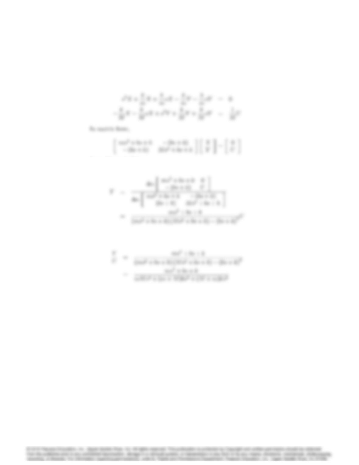
(a) The FBD for the system is

or

2013

(b) If we make Laplace Transform of the equations of motion

From Cramer’s Rule,

Finally,

9. Modify the equation of motion for the cruise control in Example 2.1,

Eq(2.4), so that it has a control law; that is, let

u=K(vrv);

where

vr= reference speed

K= constant:

This is a ‘proportional’ control law where the difference between vrand

the actual speed is used as a signal to speed the engine up or slow it down.

Put the equations in the standard state-variable form with vras the input

and vas the state. Assume that m= 1500 kg and b= 70 N s=m;and

2014 CHAPTER 2. DYNAMIC MODELS

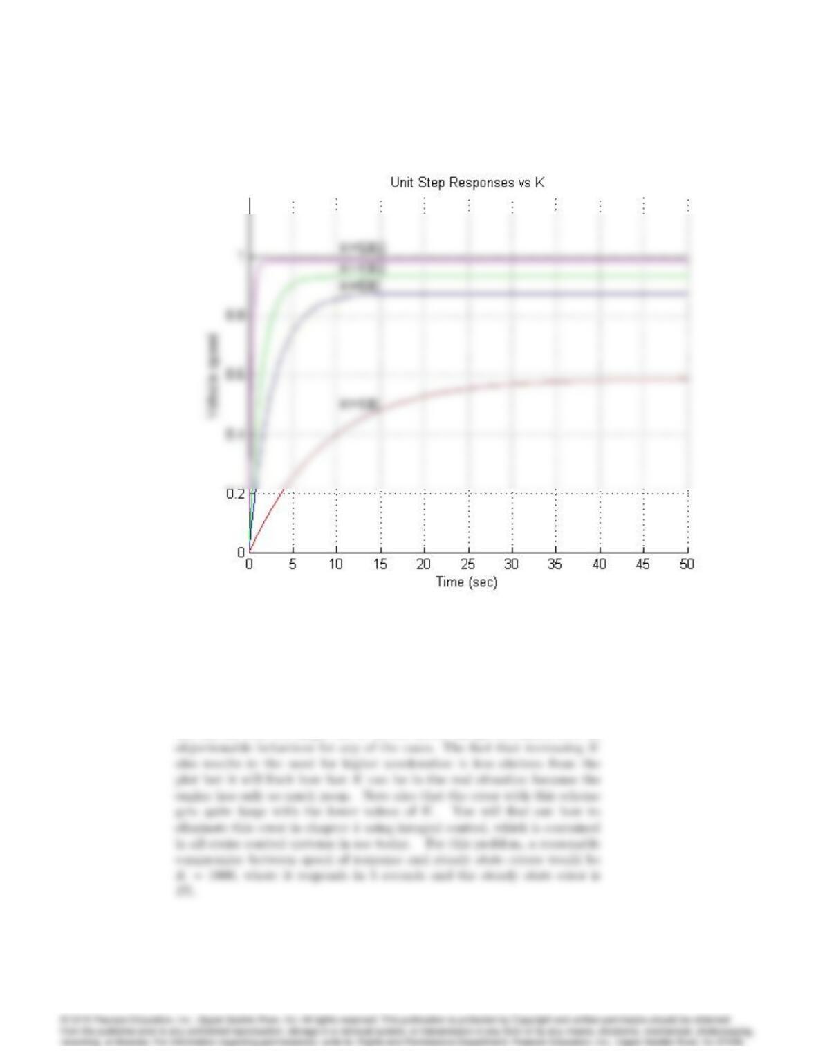
find the response for a unit step in vrusing MATLAB. Using trial and

error, find a value of K that you think would result in a control system in

which the actual speed converges as quickly as possible to the reference

speed with no objectional behavior.

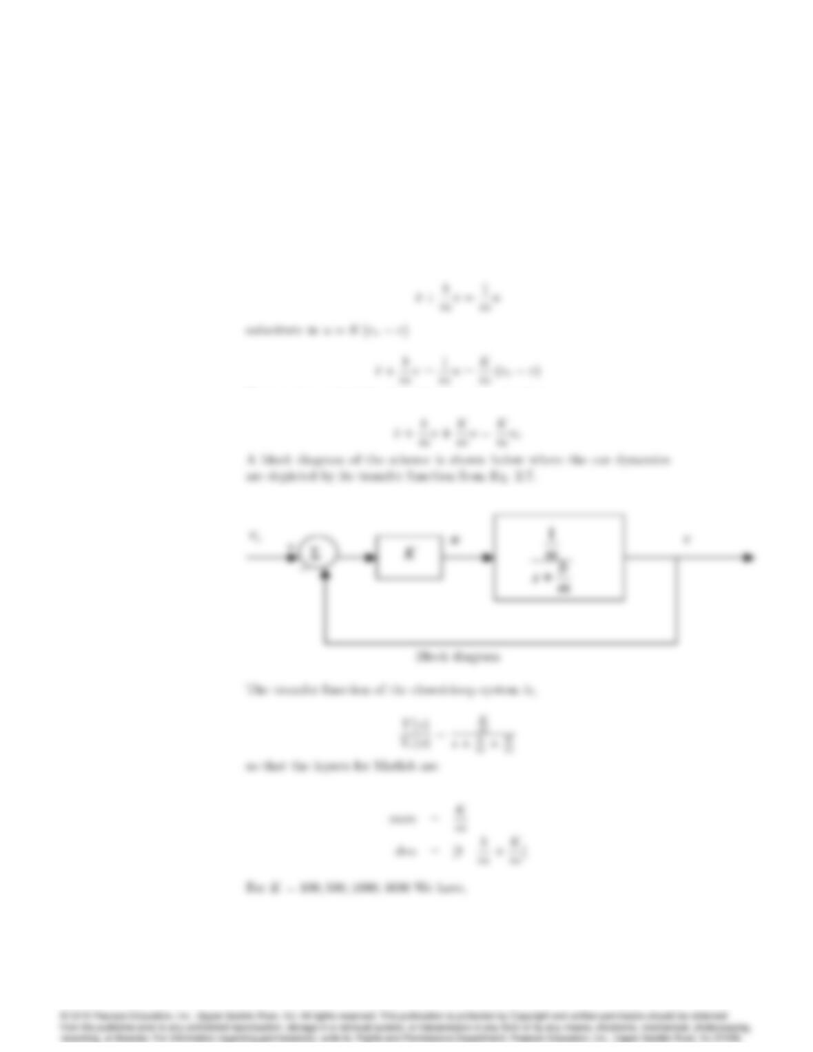
Solution:

Rearranging, yields the closed-loop system equations,

2015

We can see that the larger the Kis, the better the performance, with no

2016 CHAPTER 2. DYNAMIC MODELS

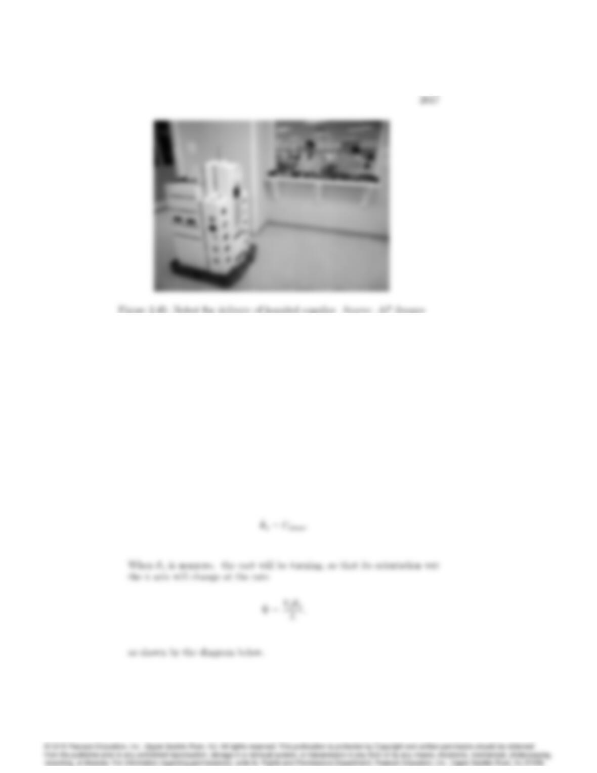
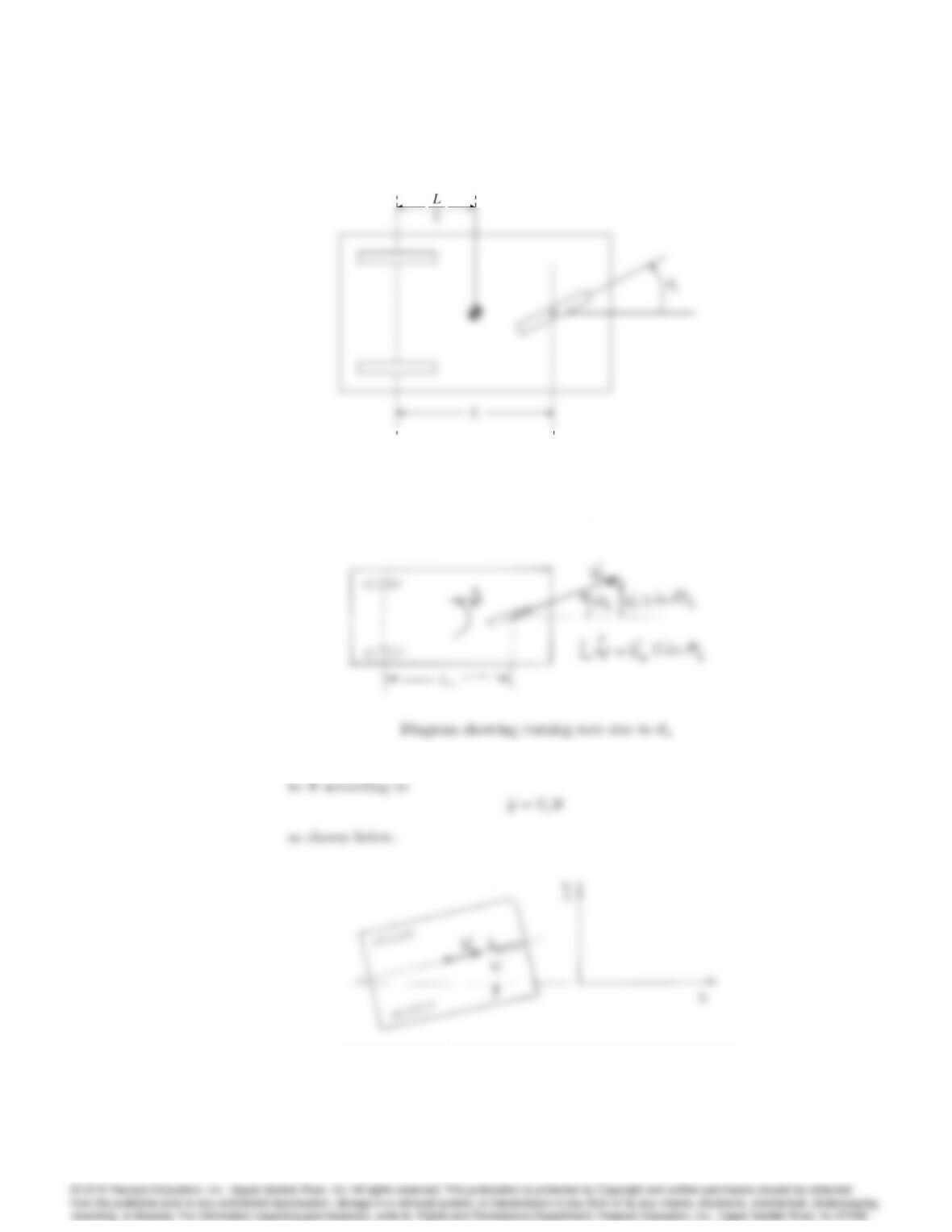
10. Determine the dynamic equations for lateral motion of the robot in Fig.

2.45. Assume it has 3 wheels with the front a single, steerable wheel

where you have direct control of the rate of change of the steering angle,

Usteer, with geometry as shown in Fig. 2.46. Assume the robot is going in

approximately a straight line and its angular deviation from that straight

line is very small Also assume that the robot is traveling at a constant

speed, Vo. The dynamic equations relating the lateral velocity of the

center of the robot as a result of commands in Usteer is desired. .

Solution:

This is primarily a problem in kinematics. First, we know that the control

input, Usteer;is the time rate of change of the steering wheel angle, so

2018 CHAPTER 2. DYNAMIC MODELS

Figure 2.46: Model for robot motion

The actual change in the carts lateral position will then be proportional

2019

Problems and Solutions for Section 2.2

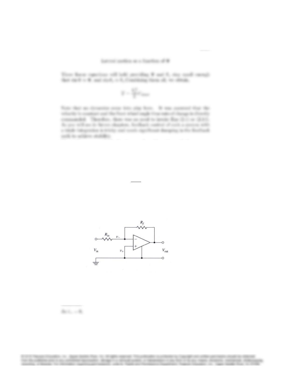
11. A first step toward a realistic model of an op amp is given by the equations

below and shown in Fig. 2.47.

Vout =107

s+ 1[V+V]

i+=i= 0

Figure 2.47: Circuit for Problem 11.

Find the transfer function of the simple amplification circuit shown using

this model.

Solution: