Operating Systems Chapter 10 Homework The Signal The Plant Noise And May

10040 CHAPTER 10. CONTROL-SYSTEM DESIGN: PRINCIPLES AND CASE STUDIES

–0.02

0.01

0.02

0.04

Root Locus

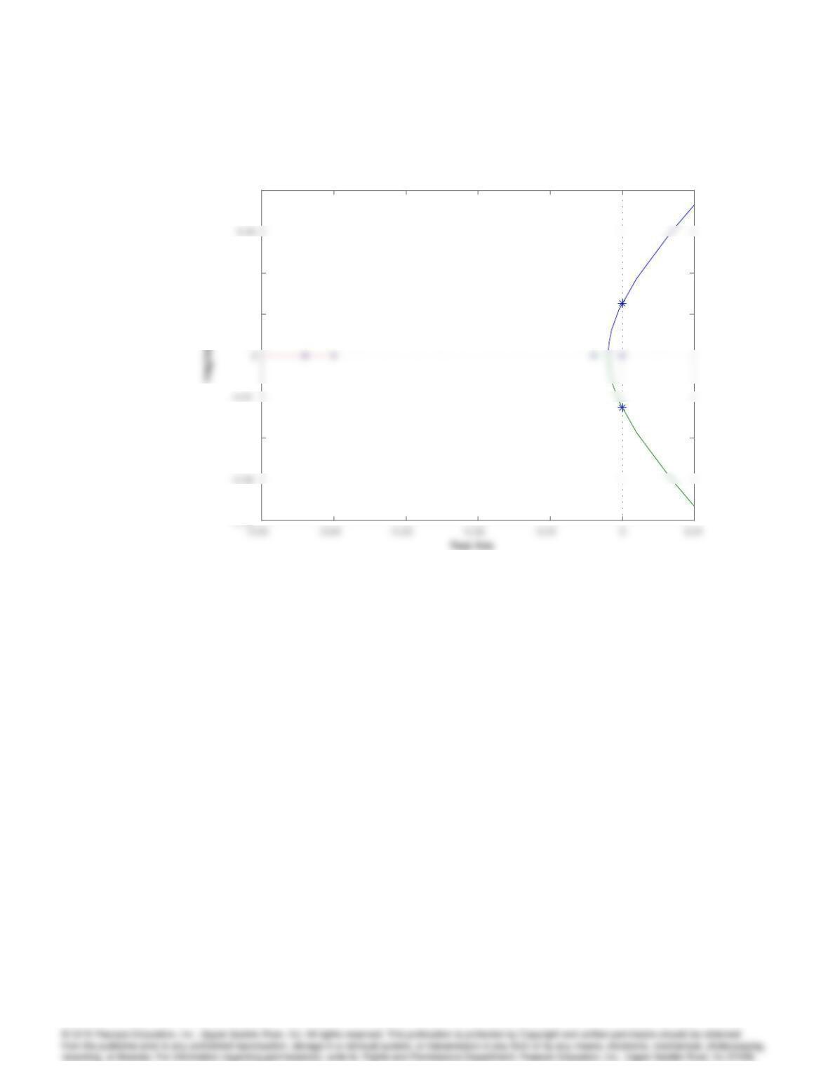
Problem 10.13: Root locus for balloon altitude control system with Dc(s) = K.

–0.3 –0.25 –0.2 –0.15 –0.1 –0.05 00.05

–0.05

0.05

0.15

Real Axis

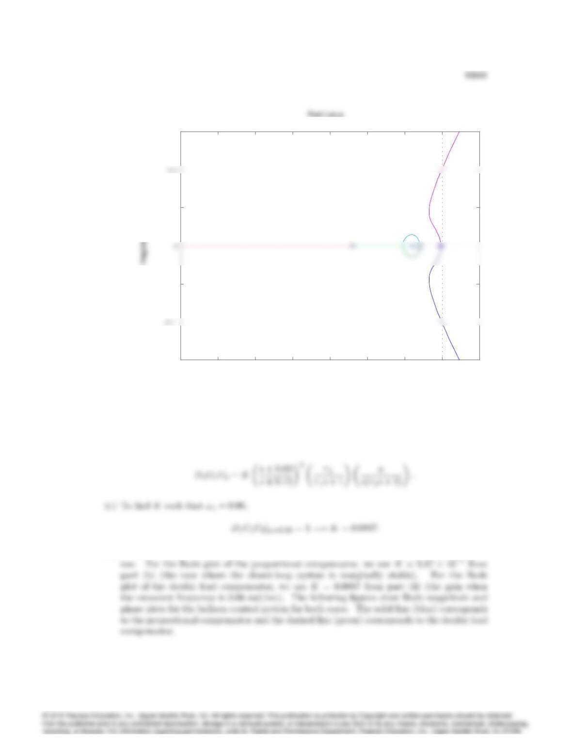
Problem 10.13: Root locus for balloon altitude control system with double-lead

compensation.

(b) The root locus using a double lead compensator is shown above. The open-loop transfer

function used is,

(d) In order to plot the Bode plots, we need to specify which values for Kwe are going to

10-3 10-2 10-1 100

–80

–40

Frequency (rad/sec)

10-3 10-2 10-1 100

–80

–40

Frequency (rad/sec)

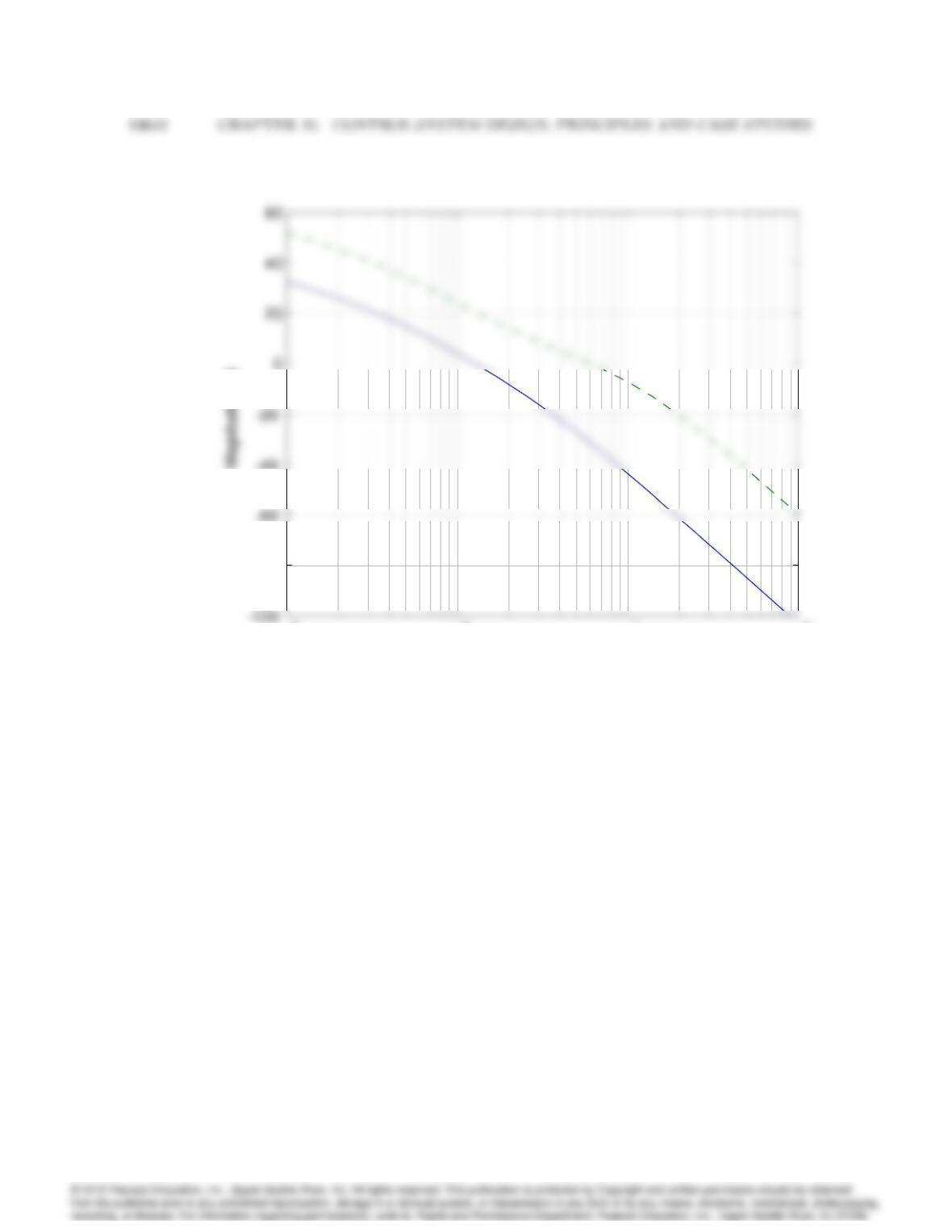
Problem 10.13: Bode magnitude plots for proportional control (blue), and double lead

compensation (green).

10-3 10-2 10-1 100

–240

–200

–160

–120

Frequency (rad/sec)

Phase (degrees)

10-3 10-2 10-1 100

–240

–200

–160

–120

Frequency (rad/sec)

Phase (degrees)

10-3 10-2 10-1 100

–240

–200

–160

–120

Frequency (rad/sec)

Phase (degrees)

10-3 10-2 10-1 100

–240

–200

–160

–120

Frequency (rad/sec)

Phase (degrees)

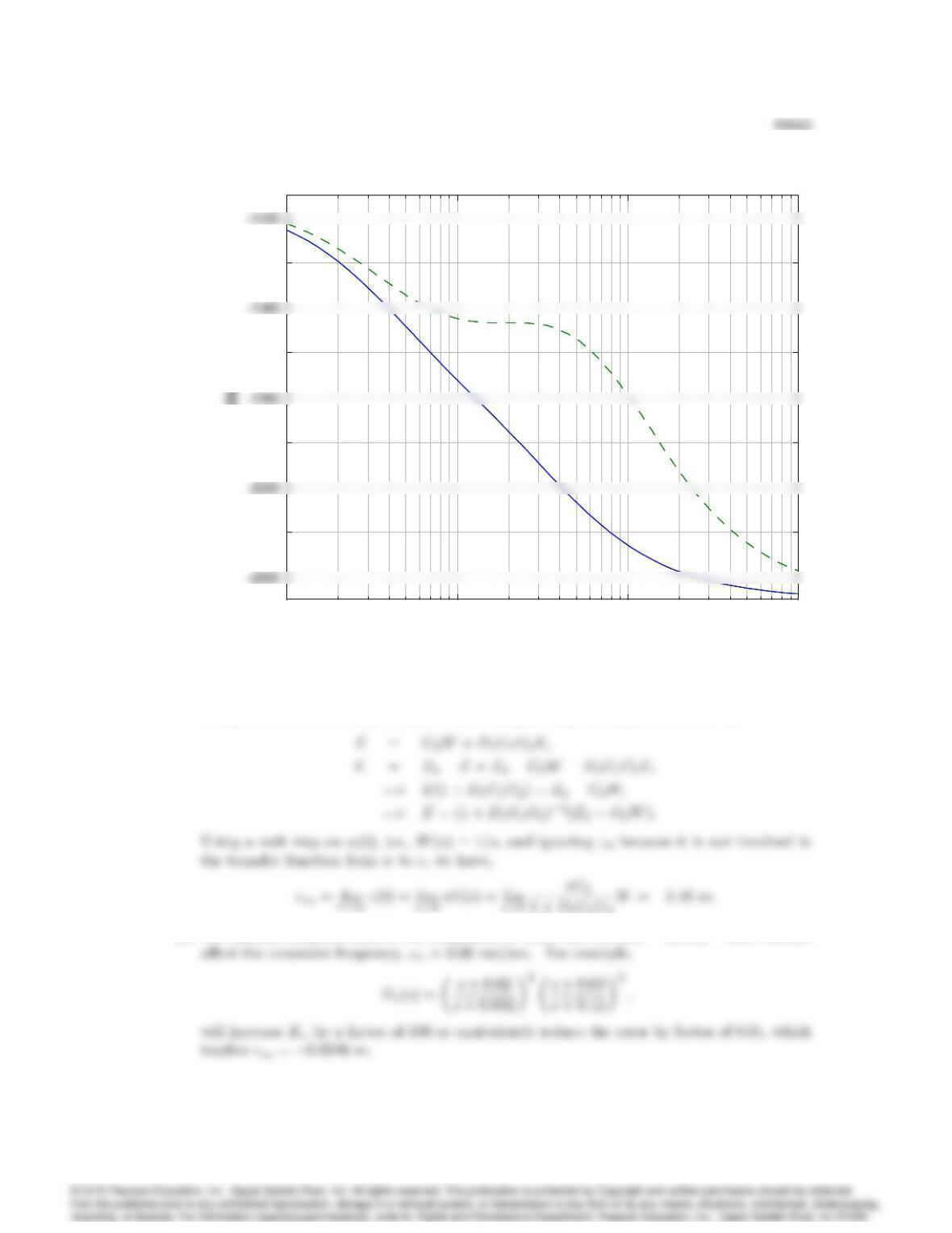
Problem 10.13: Bode phase plots for proportional control (blue), and double lead

compensation (green).

Using the notation from part (a), we have (suppressing the Laplace variable s),

(e) We can add a lag network at low frequency to boost the Kv(e1= 1=Kv). This will not

13. Satellite-attitude control systems often use a reaction wheel to provide angular motion.

The equations of motion for such a system are

Satellite :I•

=Tc+Tex;

Wheel : J_r=Tc;

Measurement : _

Z=_

aZ;

Control : Tc=D(s)(ZZd);

where,

J=moment of inertia of the wheel,

r=wheel speed,

Tc= control torque;

Tex = disturbance torque;

= angle to be controlled;

Z= measurement from the sensor;

Zd= reference angle;

I= satellite inertia (1000 kg=m2);

a= sensor constant (1 rad=sec);

Dc(s) = compensation:

(a) Suppose D(s) = K0, a constant. Draw the root locus with respect to K0for the resulting

closed-loop system.

(b) For what range of K0is the closed-loop system stable?

(c) Add a lead network with a pole at s=1so that the closed-loop system has a bandwidth

!BW = 0:04 rad=sec, a damping ratio = 0:5;and compensation given by,

Dc(s) = K1

s+z

s+ 1:

Where should the zero of the lead network be located? Draw the root locus of the com-

pensated system, and give the value of K1that allows the specifications to be met.

(d) For what range of K1is the system stable?

(e) What is the steady-state error (the difference between Zand some reference input Zd) to

a constant disturbance torque Tex for the design of part (c)?

(f) What is the type of this system with respect to rejection of Tex?

(g) Draw the Bode plot asymptotes of the open-loop system, with the gain adjusted for the

value of K1computed in part (c). Add the compensation of part (c), and compute the

phase margin of the closed-loop system.

(h) Write state equations for the open-loop system, using the state variables ,_

, and Z.

Select the gains of a state-feedback controller Tc=KK_

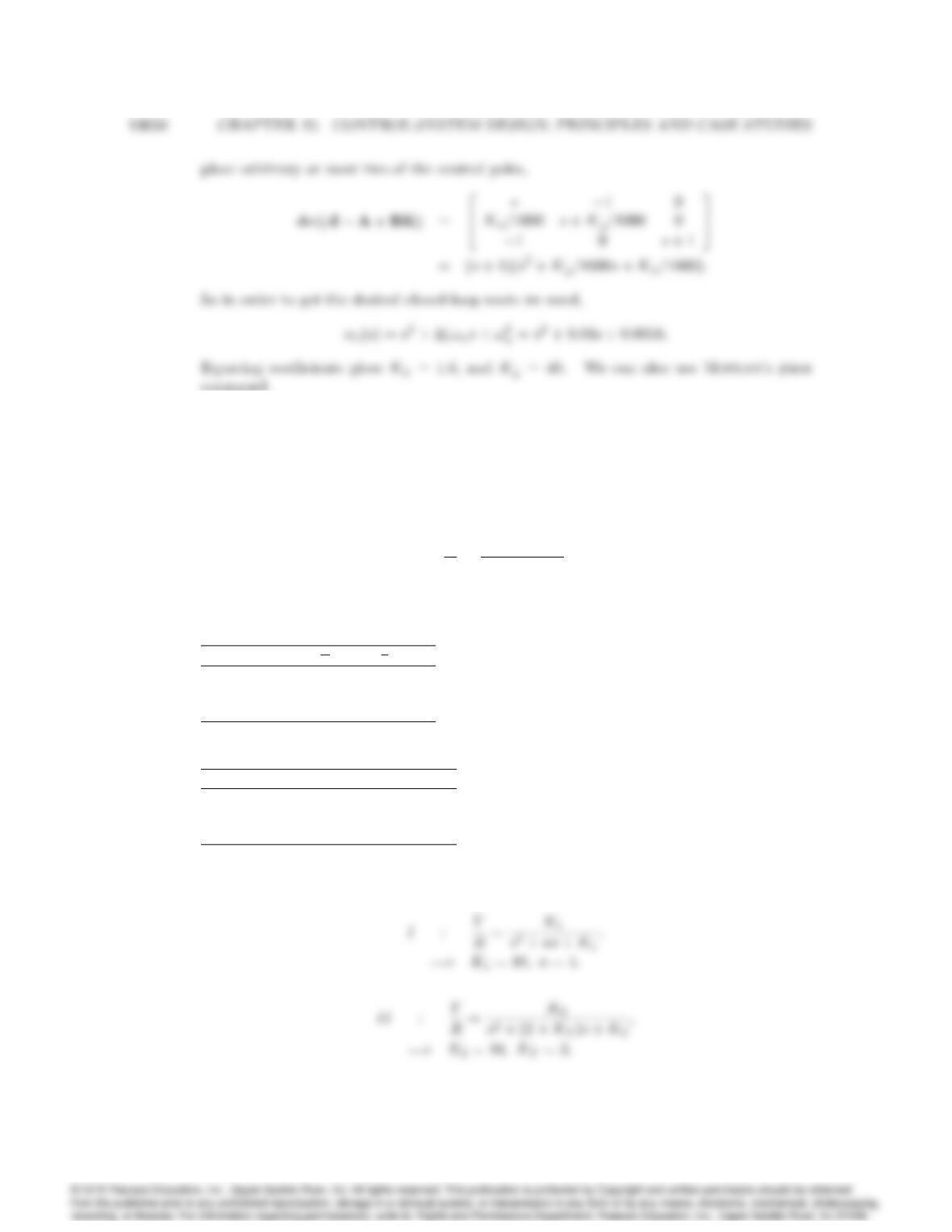
to locate the closed-loop

poles at s=0:02 0:02jp3.

Solution:

The block diagram is shown below.

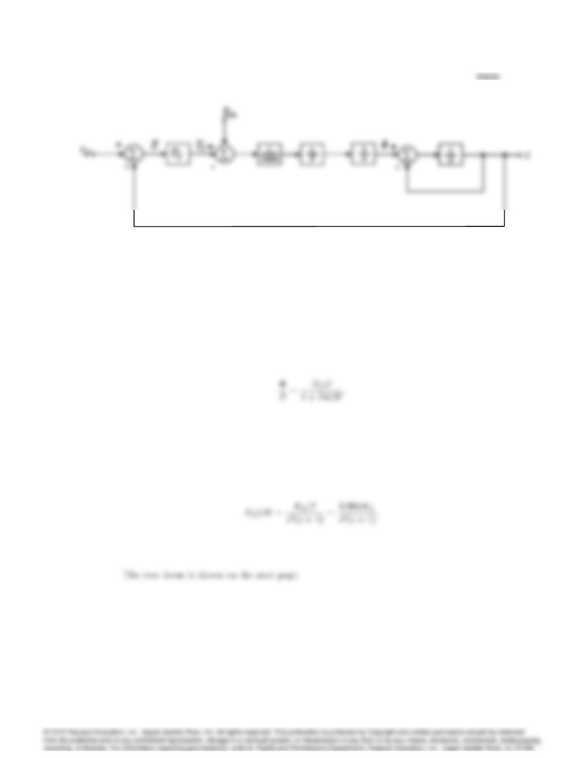
Problem 10.13: Block diagram for satellite attitude control problem.

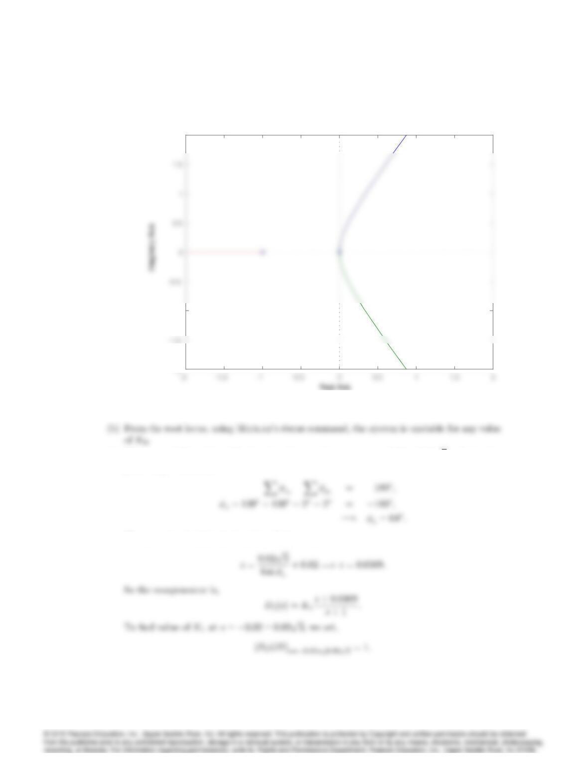
1. (a) With the transfer function from the measurement to the satellite’s angle is,

To form the root locus, we use,

10046 CHAPTER 10. CONTROL-SYSTEM DESIGN: PRINCIPLES AND CASE STUDIES

-1

2

Root Locus

Problem 10.13: Root locus for satellite problem.

(c) With !n= 0:04 and = 0:5, the closed-loop poles are at s=0:02 0:02p3j. Using the

phase angle criterion,

We can now calculate the location of the zero,

10047

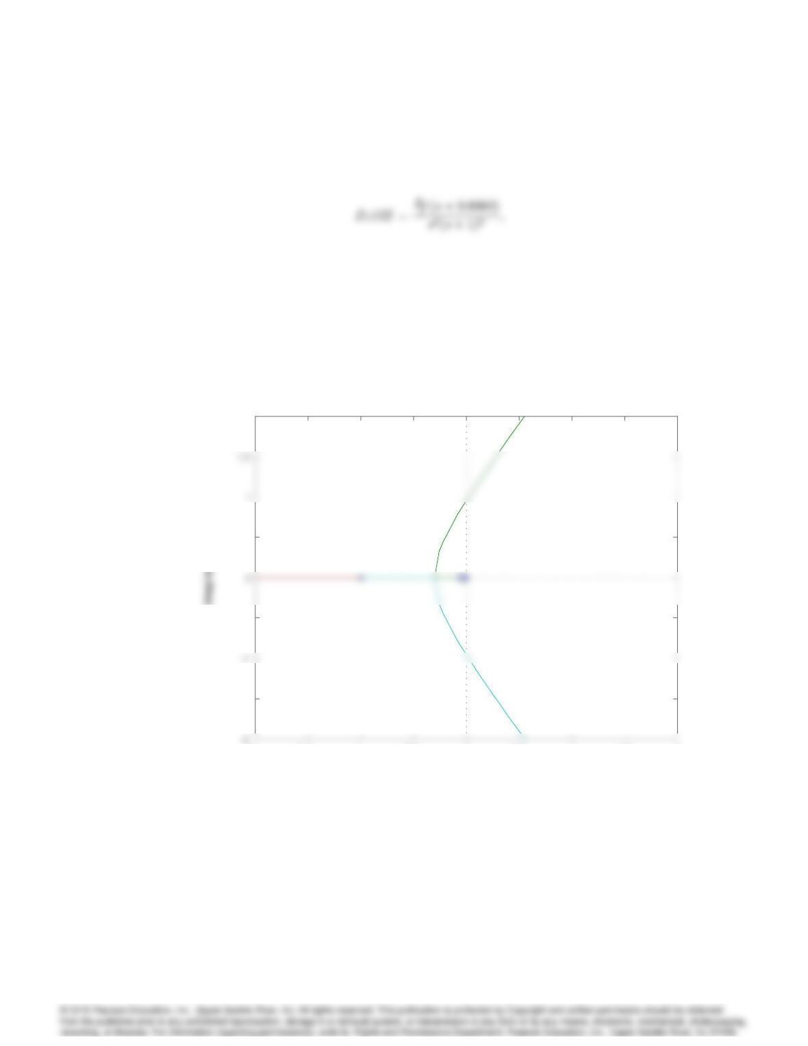
Solving for K1yields K1= 39:92. We plot the root locus of,

using Matlab’s rlocus command as shown on the next page.

-2 –1.5 -1 –0.5 00.5 11.5 2

–1.5

–0.5

0.5

2

Root Locus

Real Axis

Problem 10.13: Root locus for satellite problem with lead network.

10048 CHAPTER 10. CONTROL-SYSTEM DESIGN: PRINCIPLES AND CASE STUDIES

–0.12 –0.1 –0.08 – 0.06 – 0.04 –0.02 00.02 0.04

–0.04

Root Locus

Real Axis

Imaginary Axis

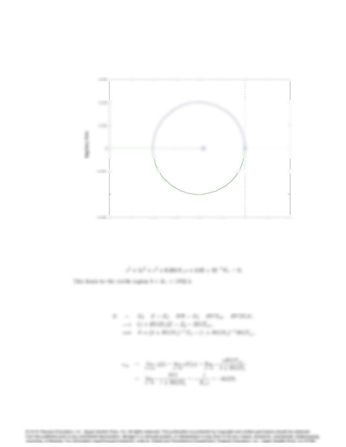
Problem 10.13: Root locus for satellite problem with lead network: detailed view.

(d) To find the range of K1for which the system is stable, we use Routh’s method on the

numerator of 1 + DcGH = 0, i.e.,

(e) We need to find the transfer function from Tex to e. In the Laplace domain (suppressing

the sfor clarity),

 = G(Tex +DcE);

Thus the steady-state error from a unit step input on Tex can be calculated using the Final

Value Theorem. With Zdand Tex = 1=s, we find,

10049

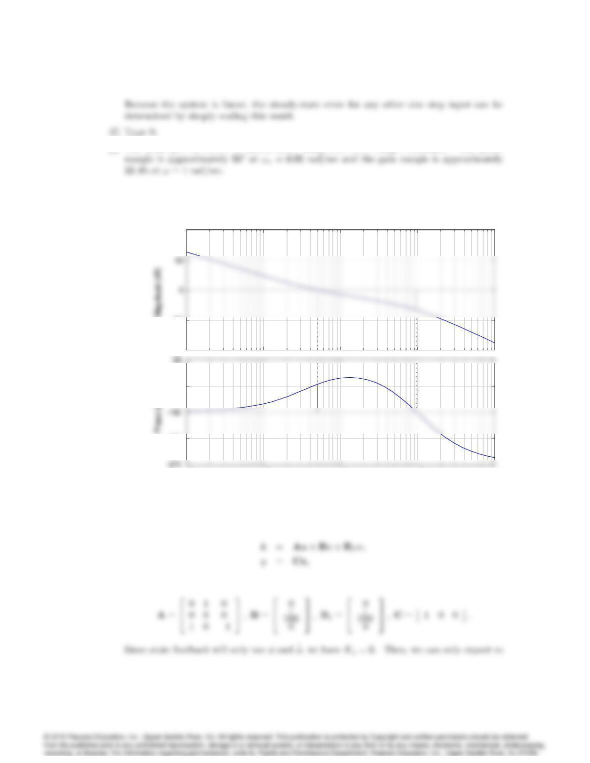
(g) The Bode plot of DcGH is shown below using Matlab’s margin command. The phase

–100

–50

100

10

-3

10

-2

10

-1

10

0

10

1

–225

–135

Bode D iag ram

Gm = 33.3 dB (at 0.962 r ad/sec) , Pm = 47.7 deg ( at 0.0496 rad/sec)

Frequency (rad/sec)

–100

–50

100

10

-3

10

-2

10

-1

10

0

10

1

–225

–135

Problem 10.13: Bode plot for satellite problem.

(h) Taking x= [x1x2x3]T= [_

 z]T,u=Tc, and w=Tex, we have,

where,

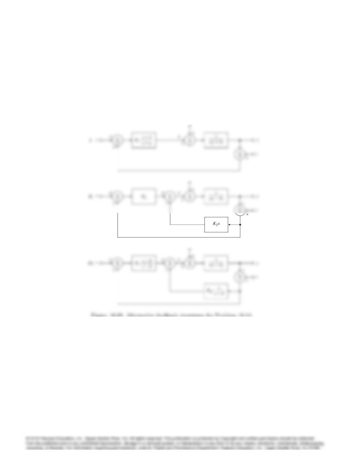
14. Three alternative designs are sketched in Fig. 10.95 for the closed-loop control of a system with

the plant transfer function G(s) = 1=s(s+ 1). The signal wis the plant noise and may be analyzed

as if it were a step; the signal vis the sensor noise and may be analyzed as if it contained power to

very high frequencies.

1. (a) Compute values for the parameters K1,a,K2,KT,K3,d, and KDso that in each case

(assuming w= 0 and v= 0),

Y

R=16

s2+ 4s+ 16:

Note that in system III, a pole is to be placed at s=4.

(b) Complete the following table, expressing the last entries as A=skto show how fast noise

from vis attenuated at high frequencies:

System Kvy

ws=0

y

vs!1

I

II

III

(c) Rank the three designs according to the following characteristics (the best as “1,” the

poorest as “3”):

I II III

Tracking

Plant-noise rejection

Sensor-noise rejection

Solution:

(a)

10051

Figure 10.95: Alternative feedback structures for Problem 10.14.

10052 CHAPTER 10. CONTROL-SYSTEM DESIGN: PRINCIPLES AND CASE STUDIES

(b) Kv:

Y

Vjs!1 :

I:Y

Filling the table, and ranking the three designs:

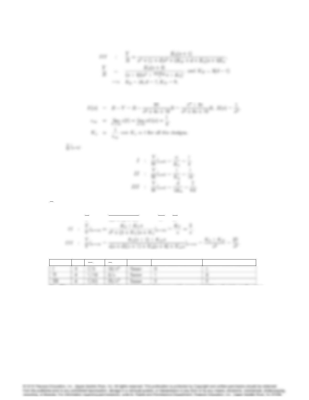
System KvY

Wjs=0 Y

Vjs!1 tracking Plant noise rejection Sensor noise rejection

15. The equations of motion for a cart-stick balancer with state variables of stick angle, stick

angular velocity, and cart velocity are

_

x=2

4

0 1 0

31:33 0 0:016

31:33 0 0:216

3

5x+2

4

0

0:649

8:649

3

5u;

y= [ 10 0 0 ]x;

where the output is stick angle, and the control input is voltage on the motor that drives the cart

wheels.

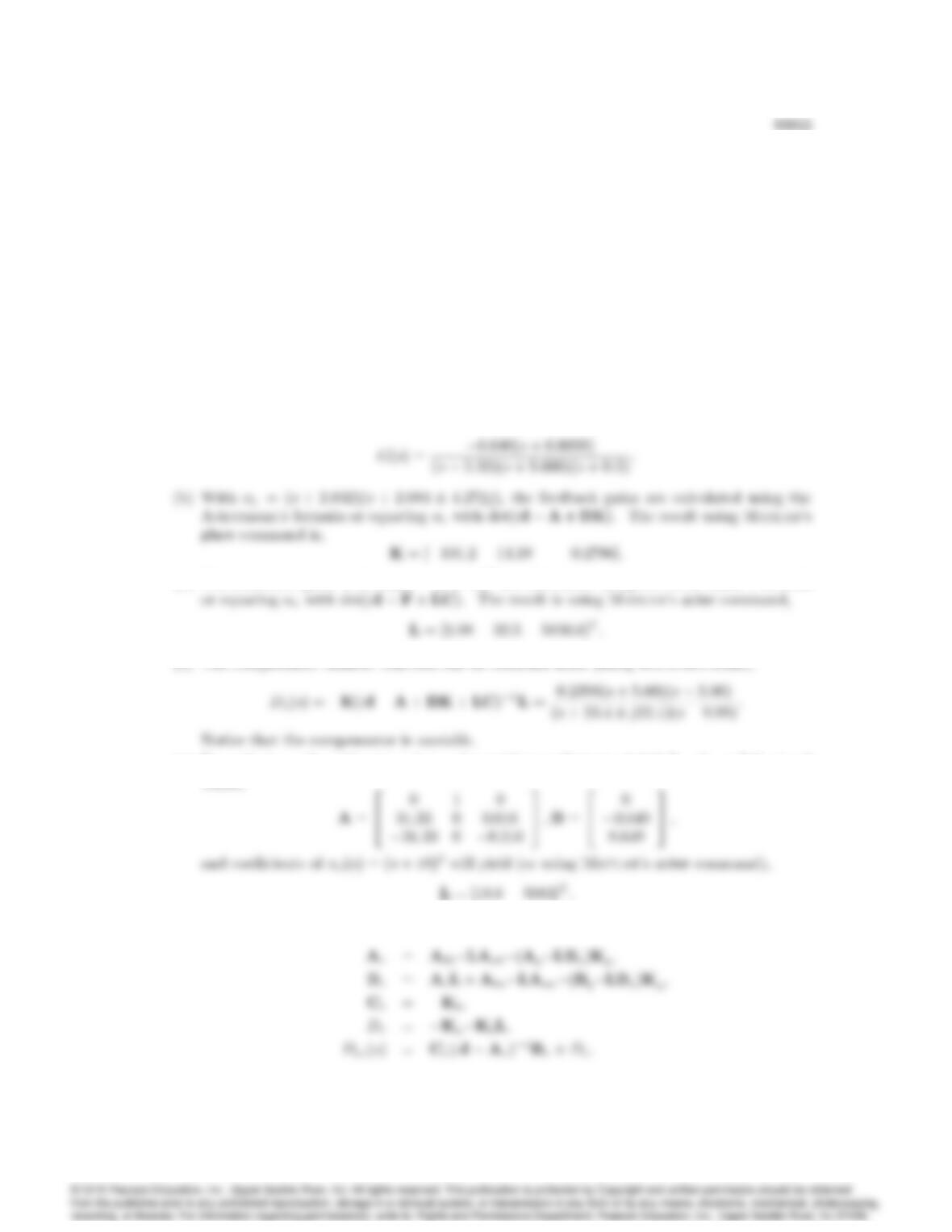
1. (a) Compute the transfer function from uto y, and determine the poles and zeros.

(b) Determine the feedback gain Knecessary to move the poles of the system to the locations

2:832 and 0:521 1:068j, with !n= 4 rad/sec.

(c) Determine the estimator gain Lneeded to place the three estimator poles at 10.

(d) Determine the transfer function of the estimated-state-feedback compensator defined by

the gains computed in parts (b) and (c).

(e) Suppose we use a reduced-order estimator with poles at 10, and 10. What is the required

estimator gain?

(f) Repeat part (d) using the reduced-order estimator.

(g) Compute the frequency response of the two compensators.

Solution:

(a) The transfer function (using Matlab’s tf) is,

(c) The estimator gains with e(s) = (s+ 10)3are calculated using the Ackermann’s formula

(e) For reducing order estimator using and matching coefficients of det(sIAbb +LAab) = 0

where,

(f) The reduced order compensator is,

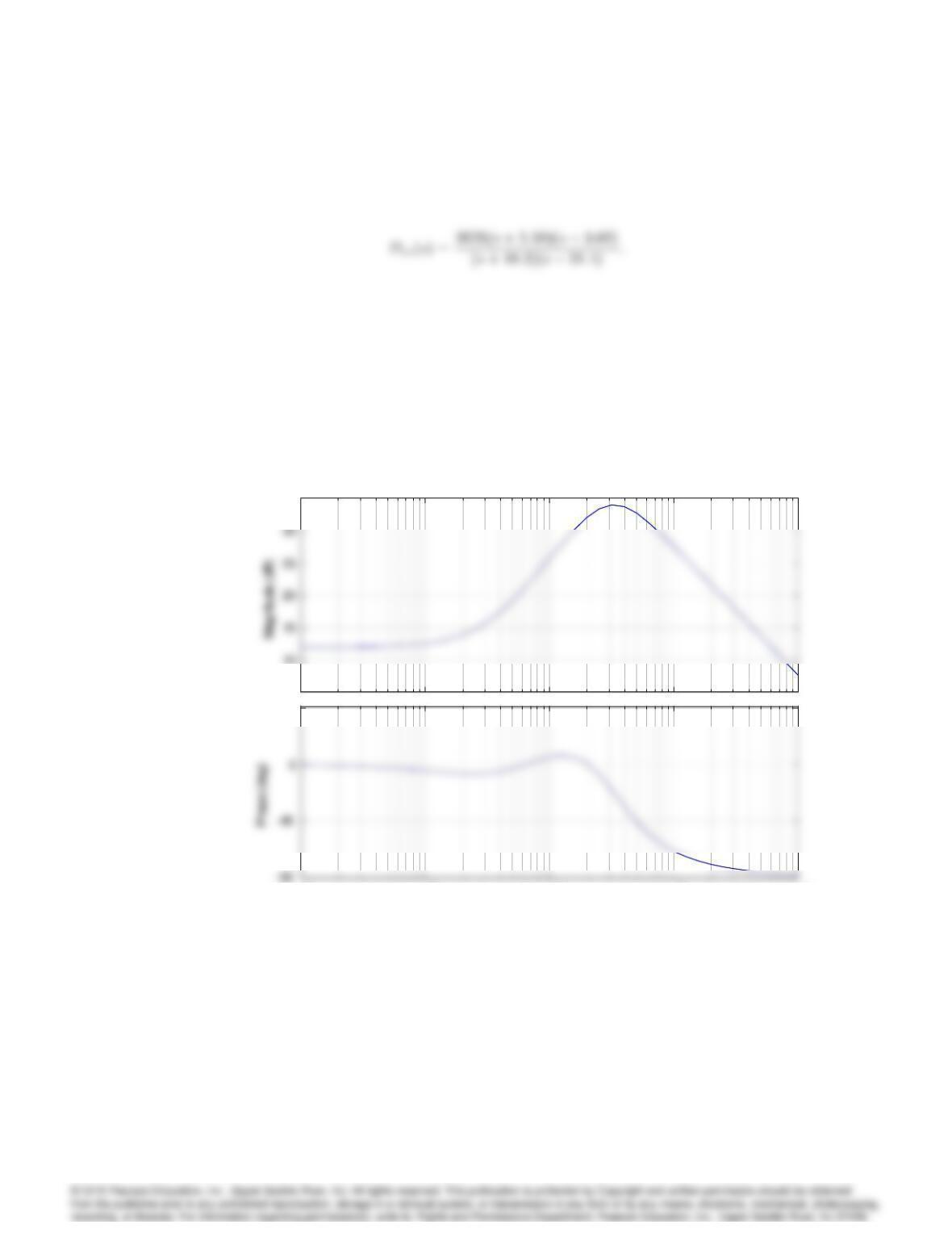
10054 CHAPTER 10. CONTROL-SYSTEM DESIGN: PRINCIPLES AND CASE STUDIES

These calculations yield (using Matlab’s ss2tf),

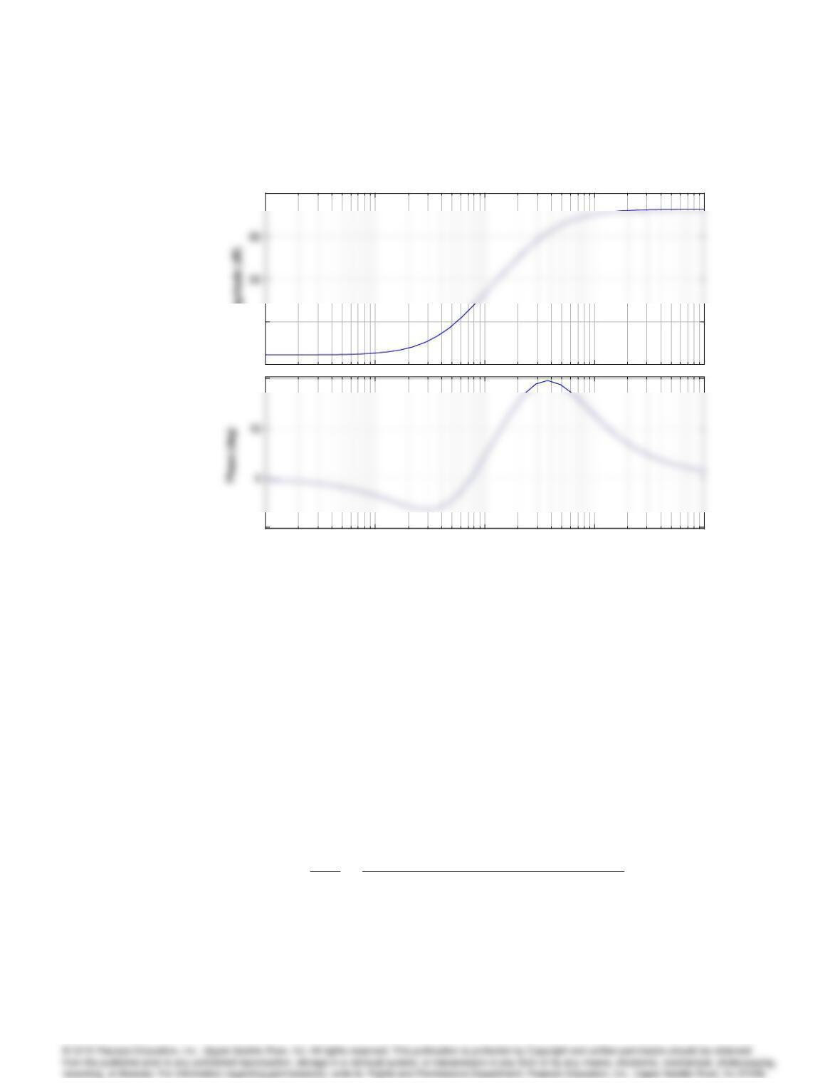
(g) The frequency responses of the two compensators follow.

5

10

35

10

-1

10

0

10

1

10

2

10

3

45

Bode D iag ram

Frequency (rad/sec)

5

10

35

10

-1

10

0

10

1

10

2

10

3

45

Frequency response of the compensator.

10055

30

40

70

Magnitude (dB)

10

-1

10

0

10

1

10

2

10

3

–10

20

Bode D iag ram

Frequency (rad/sec)

30

40

70

Magnitude (dB)

10

-1

10

0

10

1

10

2

10

3

–10

20

Frequency response of the reduced order compensator.

16. A 282-ton Boeing 747 is on landing approach at sea level. If we use the state given in

the case study (Section 10.3) and assume a velocity of 221 ft/sec (Mach 0.198), then the

lateral-direction perturbation equations are,

2

6

4

_



_r

_p

_



3

7

5=2

6

4

0:0890 0:989 0:1478 0:1441

0:168 0:217 0:166 0

1:33 0:327 0:975 0

0 0:149 1 0

3

7

52

6

4



r

p



3

7

5+2

6

4

0:0148

0:151

0:0636

0

3

7

5r;

y= [ 0100]2

6

4



r

p



3

7

5:

The corresponding transfer function is (using Matlab’s ss2tf),

G(s) = r(s)

r(s)=0:151(s+ 1:05)(s+ 0:0328 0:414j)

(s+ 1:109)(s+ 0:0425)(s+ 0:0646 0:731j):

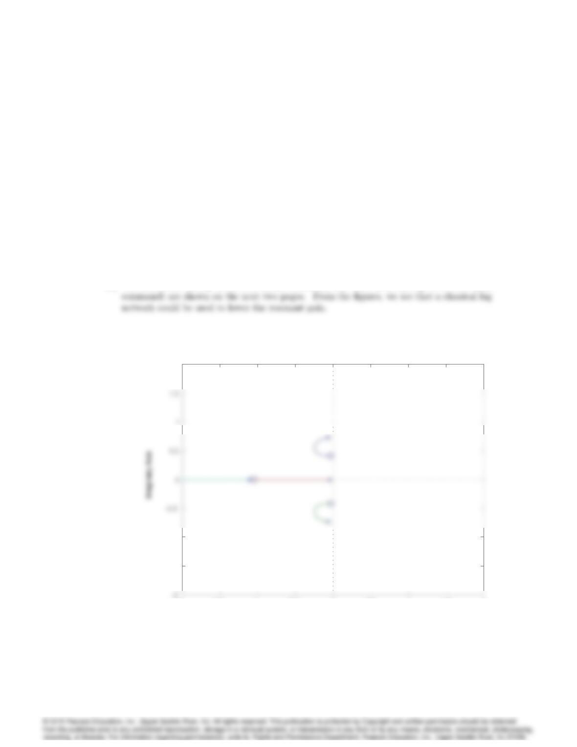
(a) Draw the uncompensated root locus [for 1 + KG(s)] and the frequency response of the

system. What type of classical controller could be used for this system?

10056 CHAPTER 10. CONTROL-SYSTEM DESIGN: PRINCIPLES AND CASE STUDIES

(b) Try a state-variable design approach by drawing a symmetric root locus for the system.

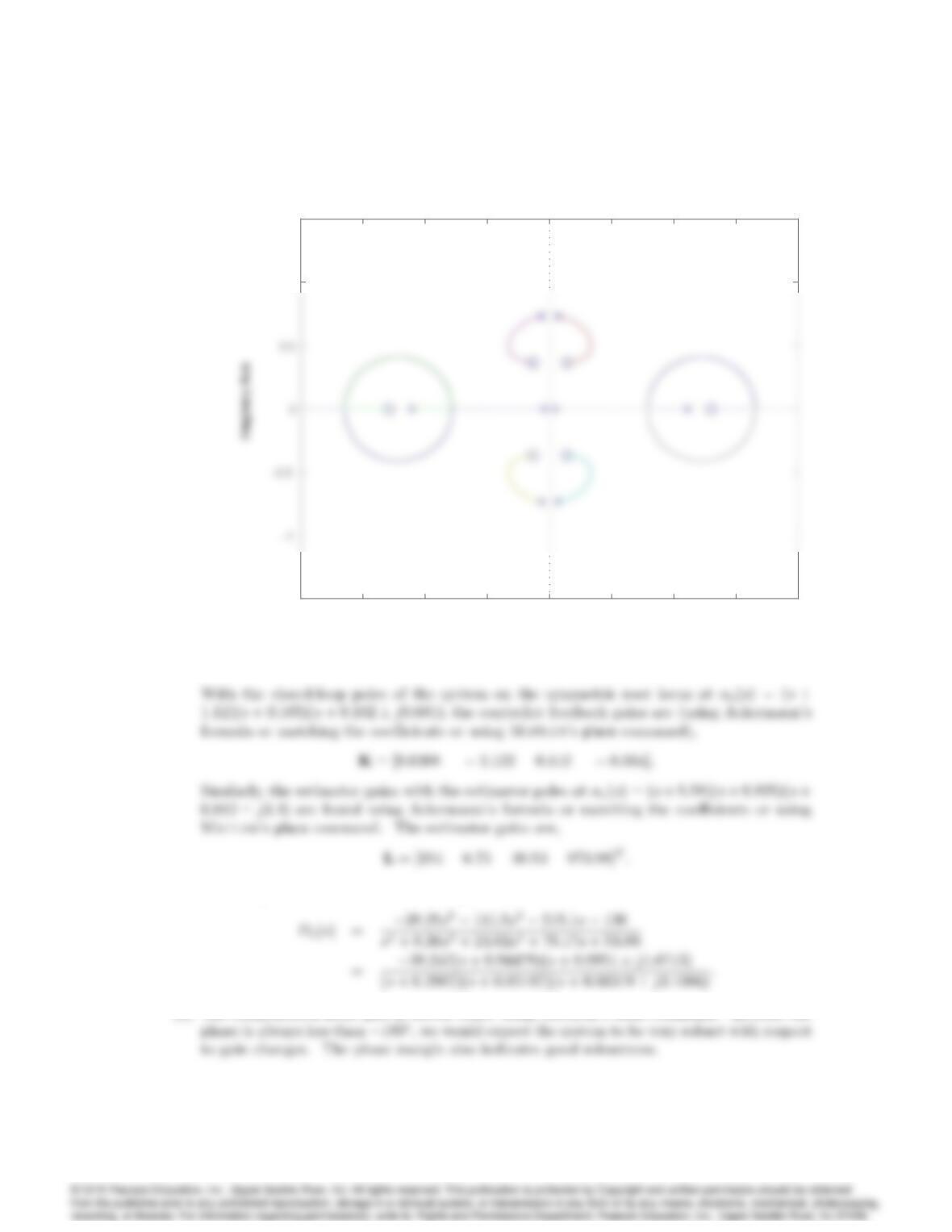
Choose the closed-loop poles of the system on the SRL to be

c(s) = (s+ 1:12)(s+ 0:165)(s+ 0:162 0:681j);

and choose the estimator poles to be five times faster at

e(s) = (s+ 5:58)(s+ 0:825)(s+ 0:812 3:40j):

(c) Compute the transfer function of the SRL compensator.

(d) Discuss the robustness properties of the system with respect to parameter variations and

unmodeled dynamics.

(e) Note the similarity of this design to the one developed for different ‡ight conditions earlier

in the chapter. What does this suggest about providing a continuous (nonlinear) control

throughout the operating envelope?

Solution:

(a) The root locus (using Matlab’s rlocus command) and Bode plots (using Matlab’s bode

-2 –1.5 -1 –0.5 00.5 11.5 2

–1.5

-1

2

Root Locus

Real Axis

Problem 10.16: Root locus for Boeing 747 problem.

10057

10-2 10-1 100101

–40

–35

–10

5

Frequency (rad/sec)

10-2 10-1 100101

–40

–35

–10

5

Frequency (rad/sec)

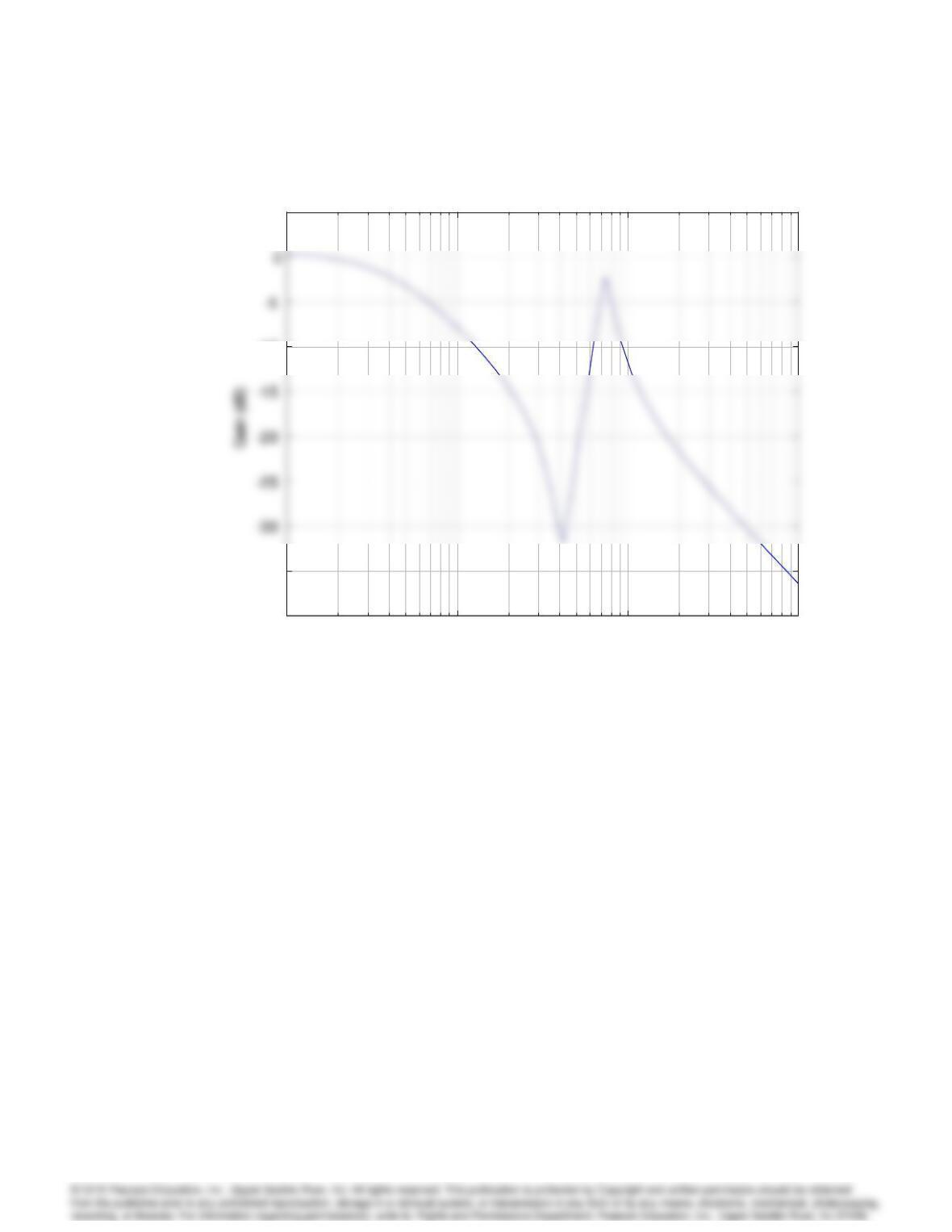
Problem 10.16: Bode magnitude plot for Boeing 747 problem.

10058 CHAPTER 10. CONTROL-SYSTEM DESIGN: PRINCIPLES AND CASE STUDIES

–100

–80

0

80

–100

–80

0

80

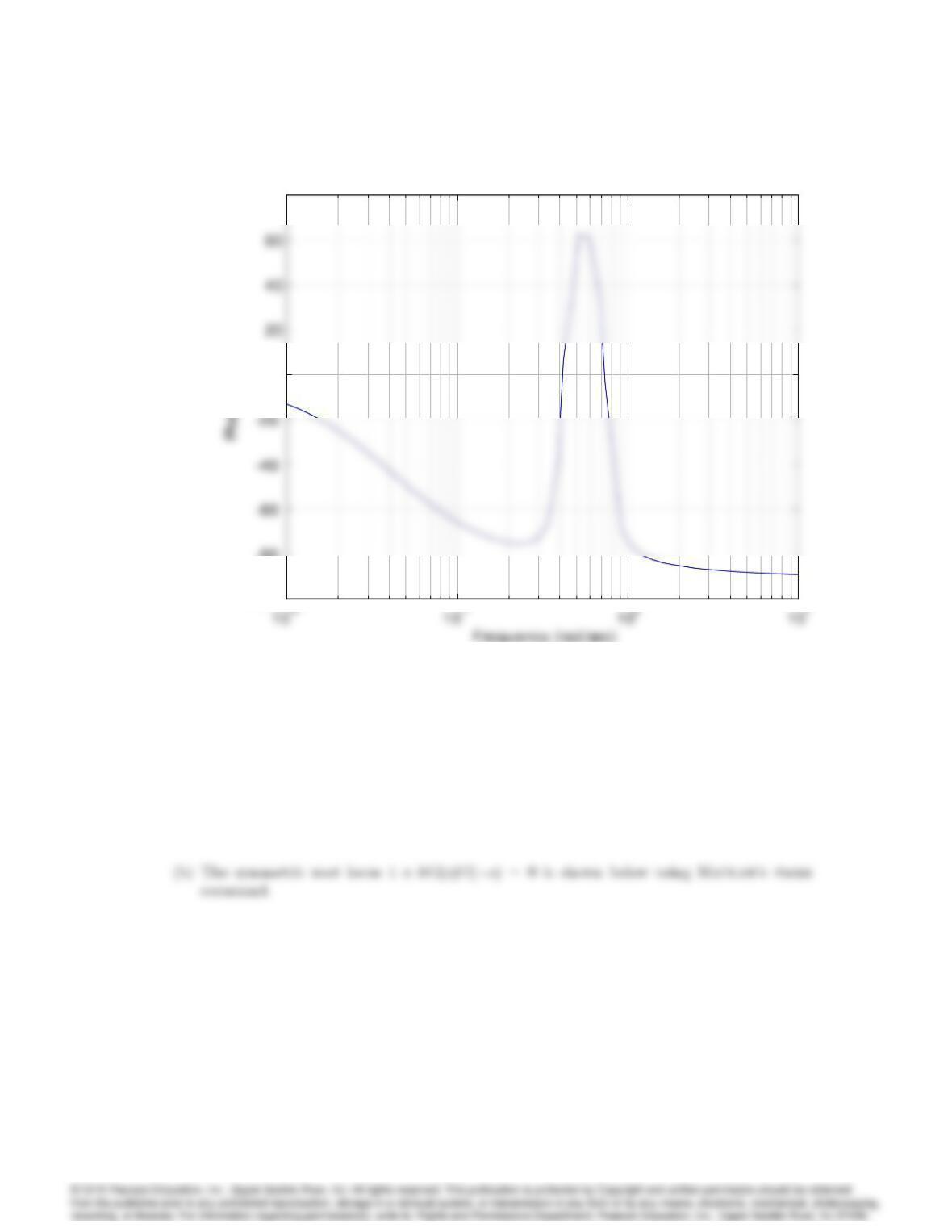
Problem 10.16: Bode phase plot for Boeing 747 problem.

10059

-2 –1.5 -1 –0.5 00.5 11.5 2

–1.5

1

1.5

Root Locus

Real Axis

Problem 10.16: Symmetric root locus for Boeing 747 problem.

(c) The compensator transfer function is given by,

(d) The compensated Bode plot is shown below using Matlab’s bode command. Because the