Operating Systems Chapter 10 Homework Let Denote The Run Number The

10060 CHAPTER 10. CONTROL-SYSTEM DESIGN: PRINCIPLES AND CASE STUDIES

–30

–20

–10

Gain dB

–30

–20

–10

Gain dB

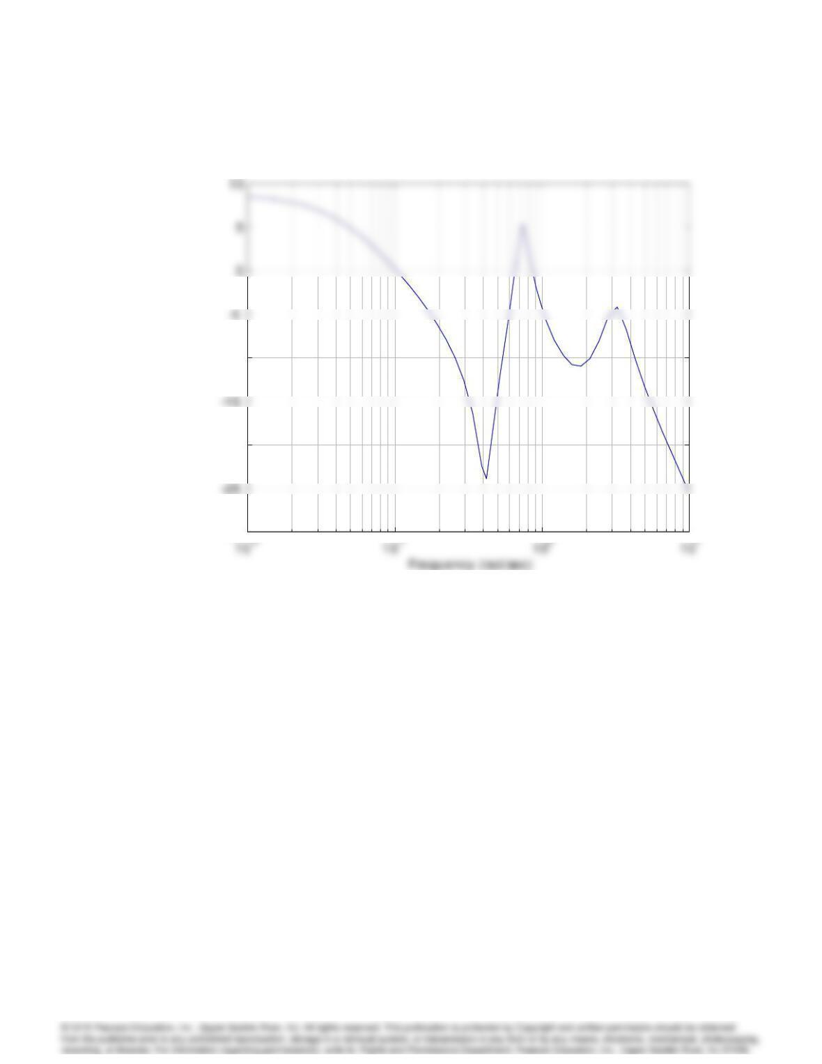
Problem 10.16: Bode magnitude for compensated system.

10061

10-2 10-1 100101

–150

100

Frequency (rad/sec)

Phase (deg)

10-2 10-1 100101

–150

100

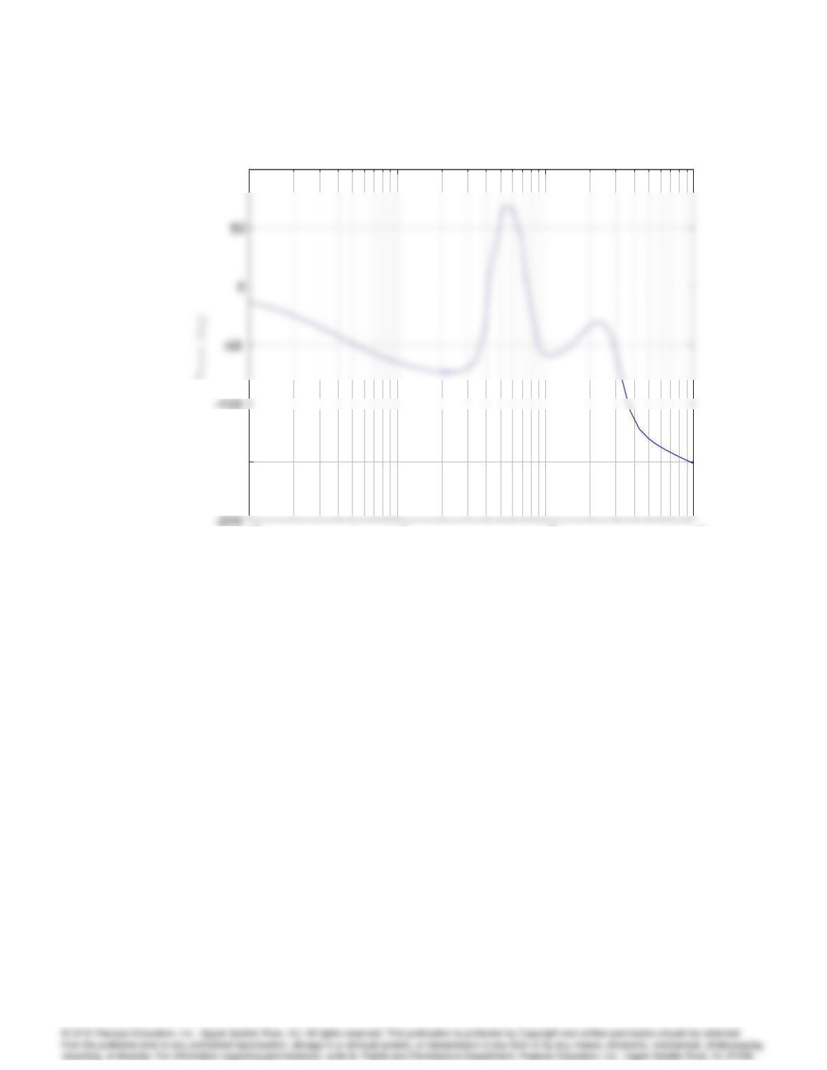
Problem 10.16: Bode phase plot for compensated system.

10062 CHAPTER 10. CONTROL-SYSTEM DESIGN: PRINCIPLES AND CASE STUDIES

–10 -8 -6 -4 -2 0 2 4 6 8 10

-8

8

10

Root Locus

Real Axis

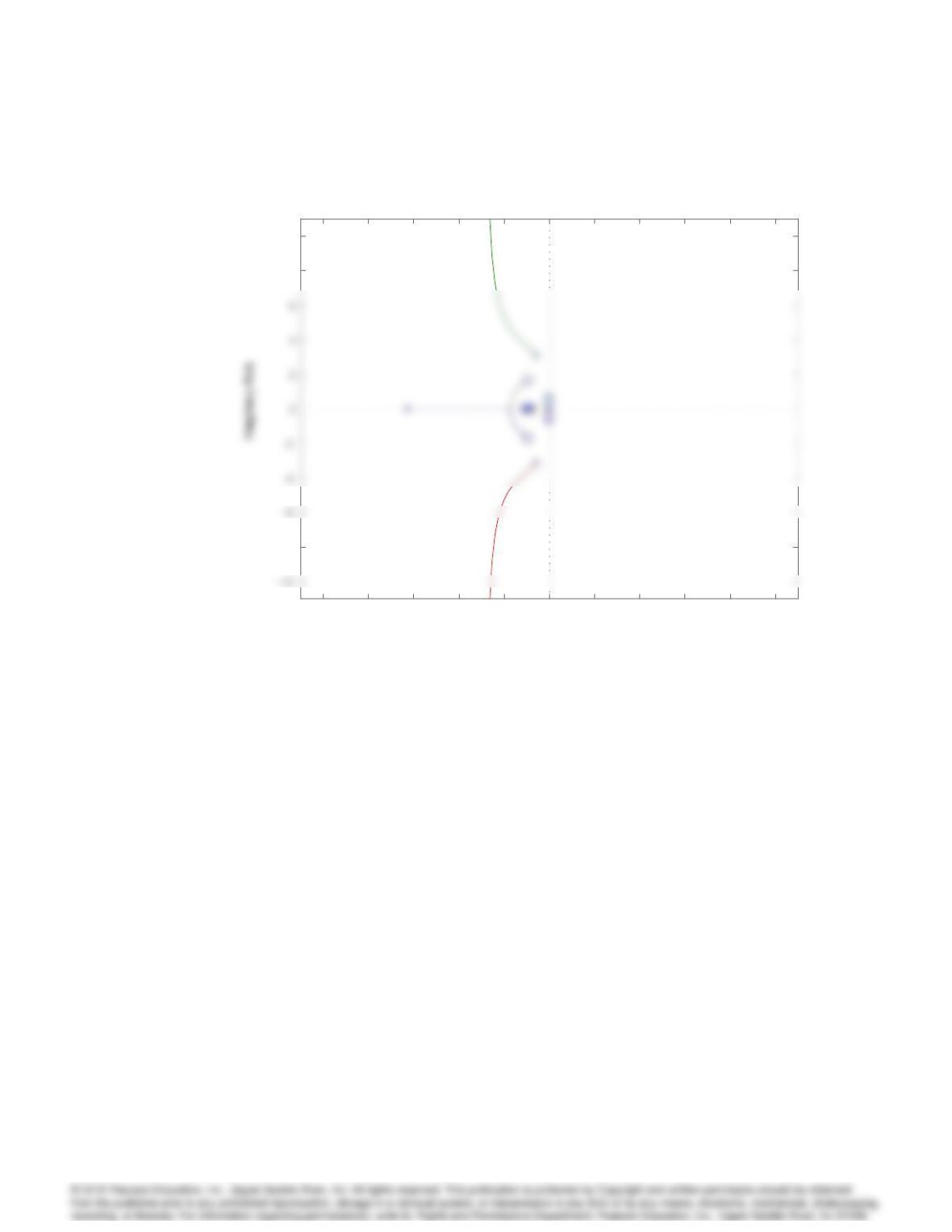
Problem 10.16: Root locus of compensated system for Boeing 747.

10063

-2 –1.5 -1 –0.5 00.5 1

–1.5

-1

1

1.5

Root Locus

Real Axis

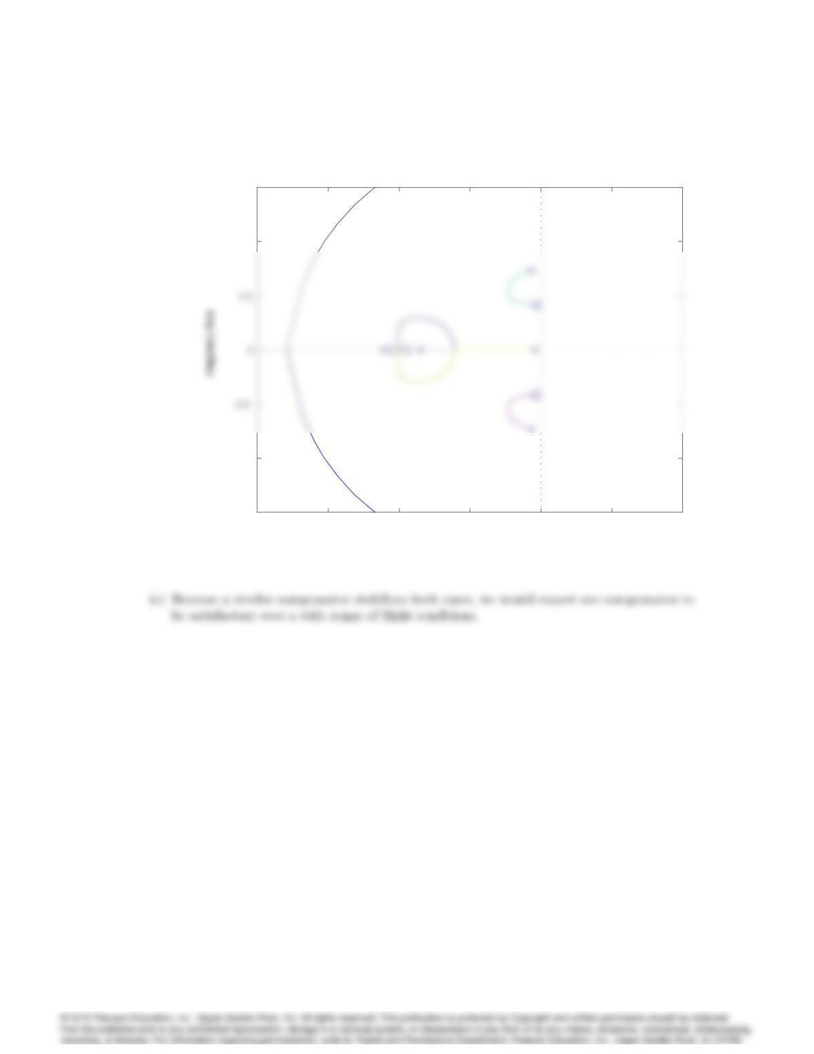
Problem 10.16 Root locus of compensated system for Boeing 747: Detailed view.

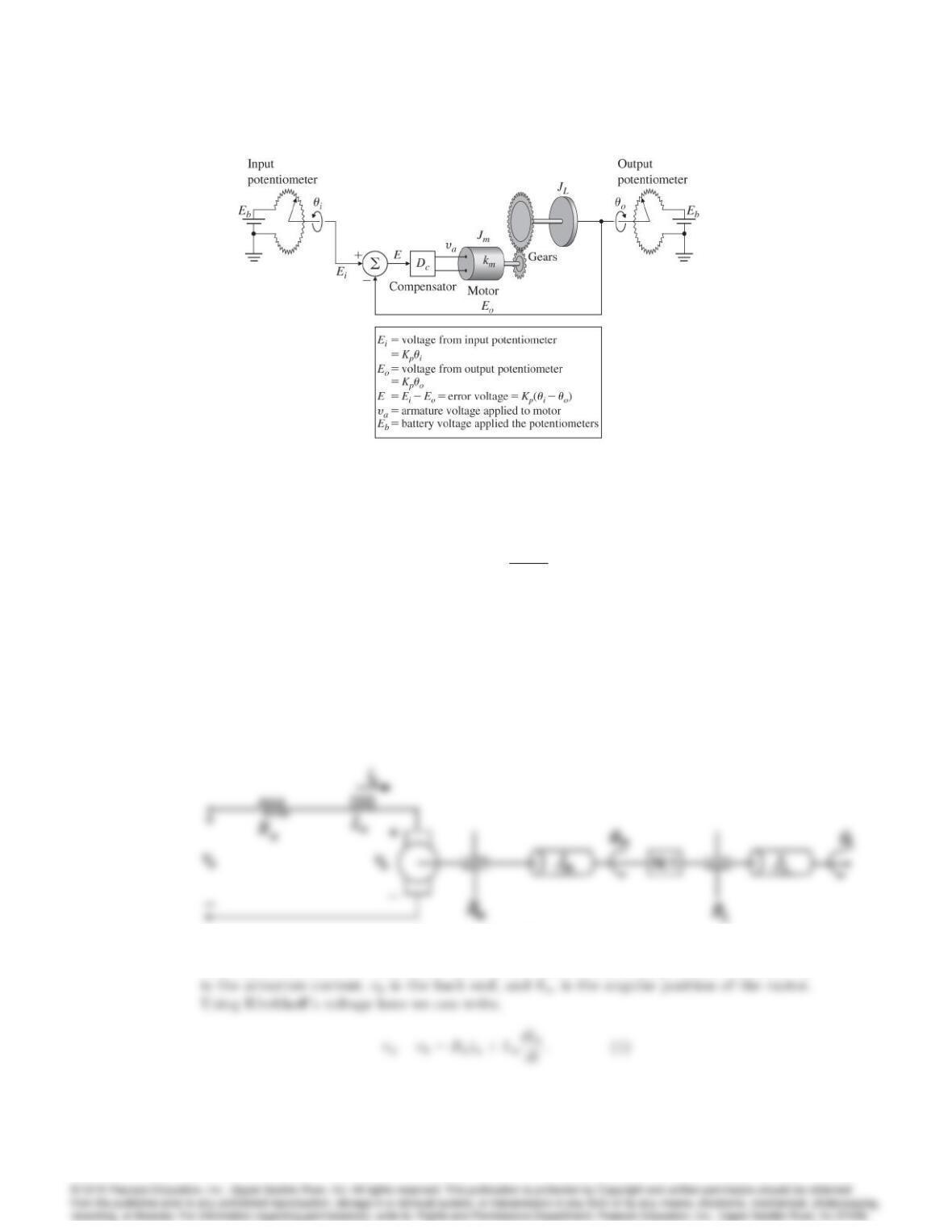
17. (Contributed by Prof. L. Swindlehurst) The feedback control system shown in Fig. 10.96 is

proposed as a position control system. A key component of this system is an armature-controlled

DC motor. The input potentiometer produces a voltage Eithat is proportional to the desired shaft

position: Ei=Kpi. Similarly, the output potentiometer produces a voltage E0that is proportional

to the actual shaft position: E0=Kp0. Note that we have assumed that both potentiometers have

the same proportionality constant. The error signal EiE0drives a compensator, which in turn

produces an armature voltage that drives the motor. The motor has an armature resistance Ra, an

armature inductance La, a torque constant Kt, and a back-emf constant Ke. The moment of inertia

of the motor shaft is Jm, and the rotational damping due to bearing friction is Bm. Finally, the gear

ratio is N: 1, the moment of inertia of the load is JL, and the load damping is BL.

1. (a) Write the differential equations that describe the operation of this feedback system.

(b) Find the transfer function relating 0(s)and i(s)for a general compensator Dc(s).

(c) The open-loop frequency-response data shown in Table 10.2 were taken using the armature

voltage vaof the motor as an input and the output potentiometer voltage E0as the output.

Assuming that the motor is linear and minimum-phase, make an estimate of the transfer

10064 CHAPTER 10. CONTROL-SYSTEM DESIGN: PRINCIPLES AND CASE STUDIES

Figure 10.96: A servomechanism with gears on the motor shaft and potentiometer sensors.

function of the motor,

G(s) = m(s)

Va(s);

where mis the angular position of the motor shaft.

(d) Determine a set of performance specifications that are appropriate for a position control

system and will yield good performance. Design Dc(s)to meet these specifications.

(e) Verify your design through analysis and simulation using Matlab.

Solution:

(a) First of all, we describe the motor dynamics in more detail. This is illustrated below.

Problem 10.17: DC motor.

The figure defines a few additional variables not mentioned in the problem statement: ia

Table 10.2: Frequency-response Data for Problem 10.17.

Frequency E0(s)

Va(s)(db)Frequency E0(s)

Va(s)(db)

(rad/sec) (rad/sec)

0.1 60.0 10.0 14.0

0.8 42.0 65.0 21.0

2.0 34.0 100.0 30.0

4.0 27.0 300.0 59.0

The torque of the motor, Tis proportional to the armature current. Thus,

The back emf, vb, is proportional to the angular speed. Hence,

At the point of contact of the gears, we assign an equal and oppositely directed force F.

(Since we do not know this force, we will eliminate it momentarily). Using Newton’s law

of motion, we have

(b) First, we will find the transfer function from vato o(the plant) and then we will find the

closed loop transfer function. From the gear ratio information, we can combine Eq. (4)

and (5) to eliminate m.

NT =NKtia= (N2Jm+JL)•

o+ (N2Bm+BL)_

o;(7)

10066 CHAPTER 10. CONTROL-SYSTEM DESIGN: PRINCIPLES AND CASE STUDIES

Thus, if we define that state x= [o_

oia]T, we have,

The output equation is y= [1 0 0]x. This state space realization can then be converted

to transfer function form. We find,

And so the closed-loop transfer function is,

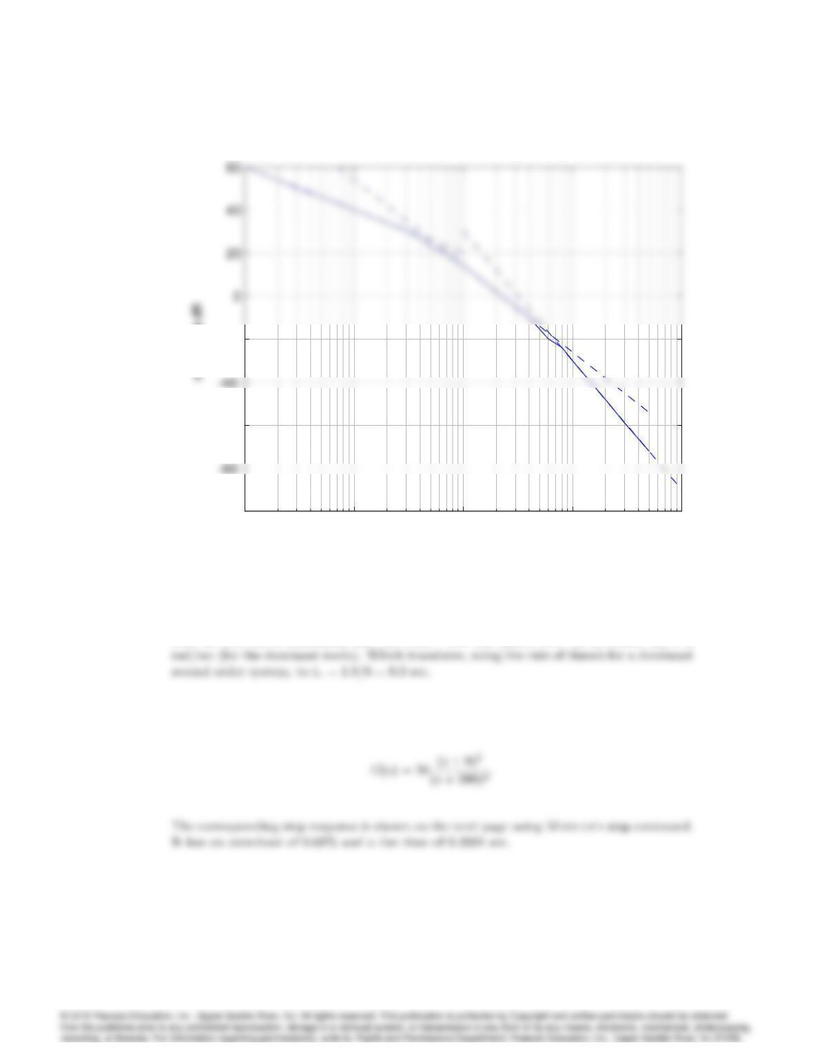
(c) The figure on the next page shows three straight lines fit through the frequency response

data. From this information, we can estimate the transfer function of the plant, G(s).

From the figure, the poles appear to be located at != 5 rad/sec and != 70 rad/sec.

Keeping the sign convention from part (b), we have,

The gain, =La, is determined by picking a particular value of !, say != 1, comparing

the calculated transfer function with the frequency response data. We find,

10067

10-1 100101102103

–100

–60

–20

ω rad/sec

10-1 100101102103

–100

–60

–20

ω rad/sec

Problem 10.17: Straight line fits to frequency response.

(d) For a positioning system, we would like to keep the overshoot small, less than 1% (say).

And we also like a reasonably fast rise time. For this plant, let’s try to obtain !n= 6

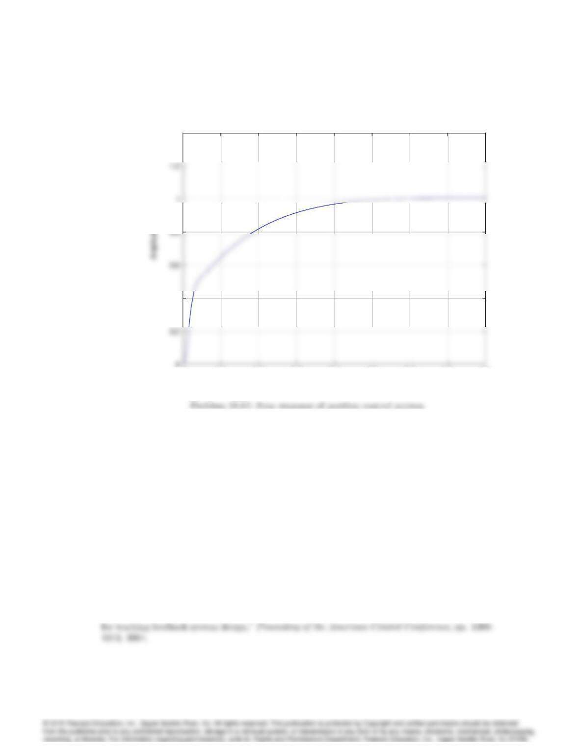
(e) Both of the time domain specifications are met using a double lead compensator,

10068 CHAPTER 10. CONTROL-SYSTEM DESIGN: PRINCIPLES AND CASE STUDIES

00.1 0.2 0.3 0.4 0.5 0.6 0.7 0.8

0.4

1.4

Step Response

Time (sec)

00.1 0.2 0.3 0.4 0.5 0.6 0.7 0.8

0.4

1.4

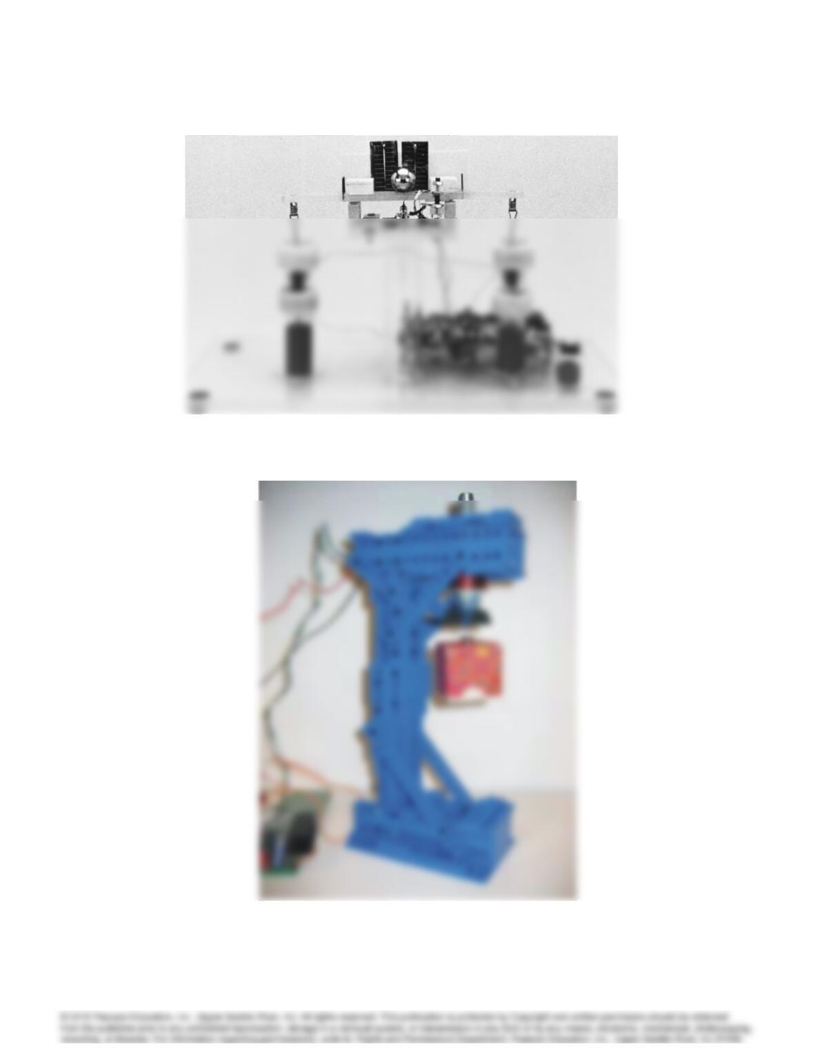
18. Design and construct a device to keep a ball centered on a freely swinging beam.

An example of such a device is shown in Fig. 10.97. It uses coils surrounding permanent

magnets as the actuator to move the beam, solar cells to sense the ball position, and a hall-

effect device to sense the beam position. Research other possible actuators and sensors as

part of your design effort. Compare the quality of the control achievable for ball-position-

feedback only with that of multiple-loop feedback of both ball and beam position.

Solution:

See Text Figure 10.97.

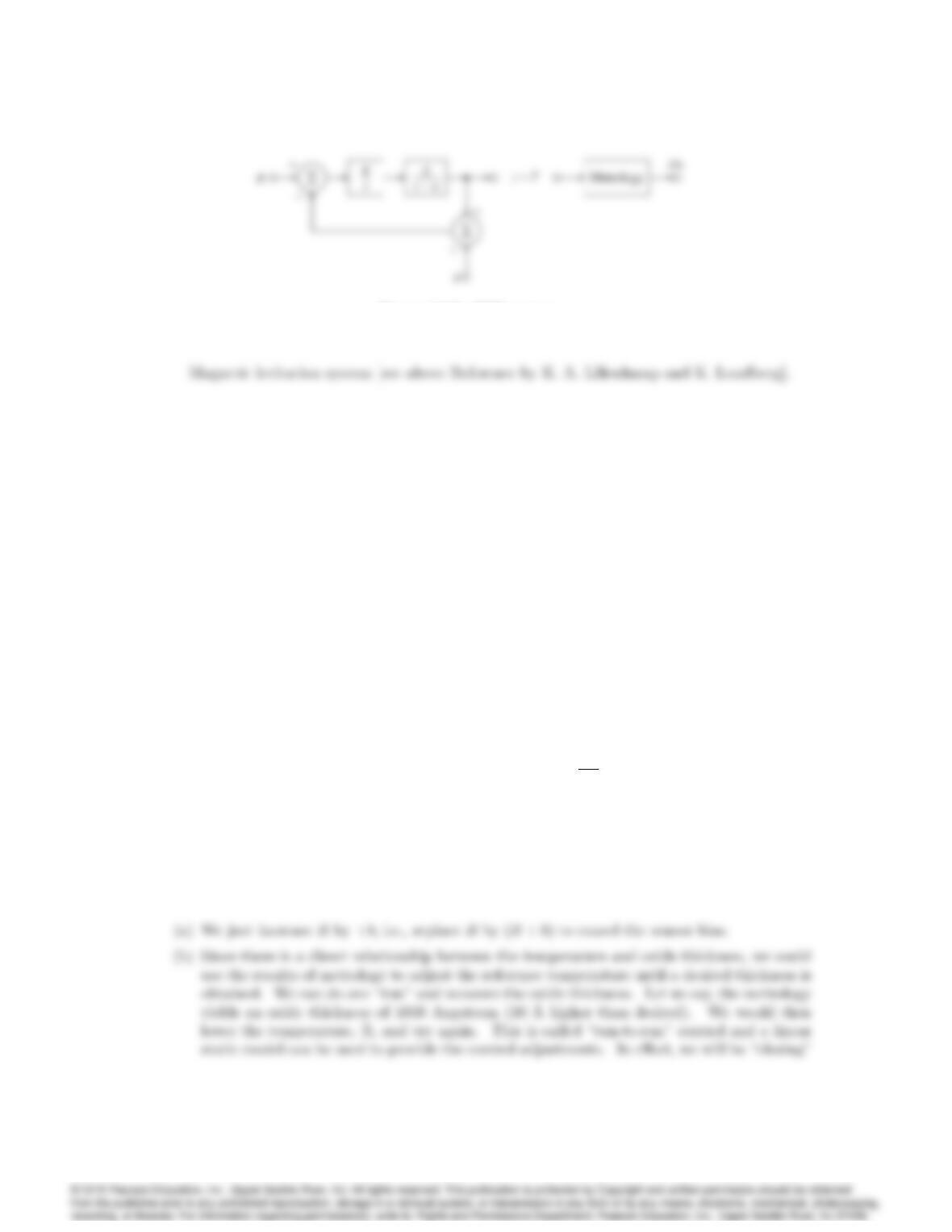
19. Design and construct the magnetic levitation device shown in Figure 9.2. You may wish to

use LEGO components in your design.

1. Solution: see K. A. Lilienkamp and K. Lundberg,“Low-cost magnetic levitation project kits

10069

Figure 10.97: Ball-balancer design example.

10070 CHAPTER 10. CONTROL-SYSTEM DESIGN: PRINCIPLES AND CASE STUDIES

Figure 10.98: RTP system.

20. Design and build a Sun tracker using an Arduino board and related software.

Solution: See several prototypes on the Internet.

21. Run-to-Run Control: Consider the rapid thermal processing (RTP) system shown in Fig. 10.98.

We wish to heat up a semiconductor wafer, and control the wafer surface temperature accurately using

rings of tungsten halogen lamps. The output of the system is temperature Tas a function of time,

y=T(t). The system reference input Ris a desired step in temperature (700C) and the control

input is lamp power. A pyrometer is used to measure the wafer center temperature. The model of

the system is first order and an integral controller is used as shown in Figure 10.98. Normally, there

is not a sensor bias (b= 0).

a. Suppose the system suddenly develops a sensor bias b6= 0, where bis known. What can be done

to ensure zero steady-state tracking of temperature command Rdespite the presence of the sensor

bias?

1. (a) Now assume b= 0. In reality, we are trying to control the thickness of the oxide film

grown (Ox) on the wafer and not the temperature. At present no sensor can measure Ox

in real time. The semiconductor process engineer must use an off-line equipment (called

metrology) to measure the thickness of the oxide film grown on the wafer. The relationship

between the system output temperature and Ox is nonlinear and given by

Oxide thickness =Ztf

0

pec

T(t)dt;

where tfis the process duration, and pand care known constants. Suggest a scheme

in which the center wafer oxide thickness Ox can be controlled to a desired value (say,

Ox = 5000 Å) by employing the temperature controller and the output of the metrology.

Solution:

10071

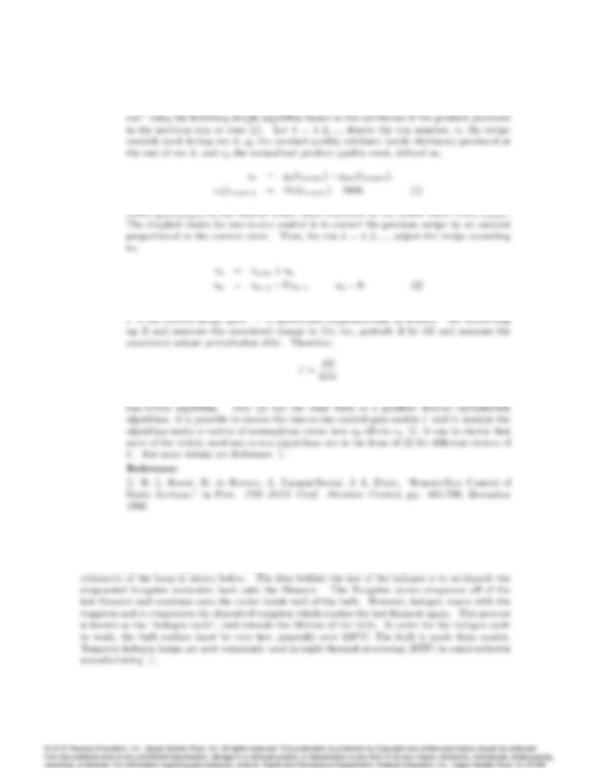
the loop on metrology with a discrete integrator [1]. The recipe is adjusted from “run-to-

where rnom is the nominal recipe, ukis the correction to the nominal recipe for run k, and

is the control design gain. It is important to emphasize that (1)-(2) constitute the complete

22. Develop a nonlinear model for a tungsten halogen lamp and simulate it in Simulink.

Solution:

Discovered in 1959, a tungsten halogen bulb is similar to an ordinary incandescent bulb with the

filament made from tungsten but the fill gas is a halogen compound, usually iodine or bromine. A

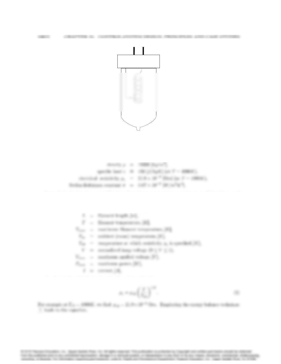
Problem 10.21: Schematic of a tungsten halogen lamp.

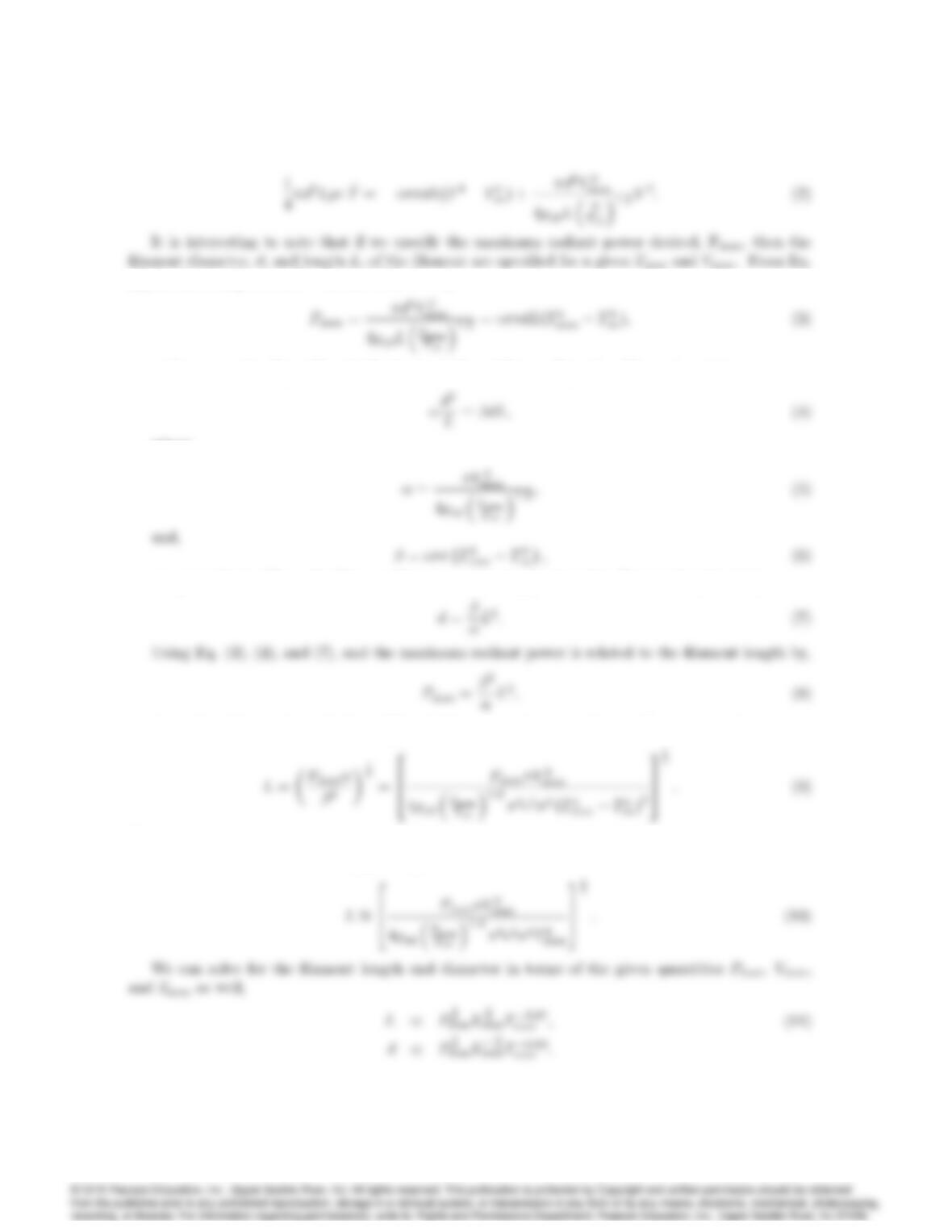
Consider the following physical parameters for the lamp,

total emissivity 

=0:4;

Lamp design is based on a specification of maximum temperature, maximum applied voltage, and

maximum delivered power. Using the following notation,

d=filament diameter;[mm];

the electrical resistivity is given by the relationship [3],

10073

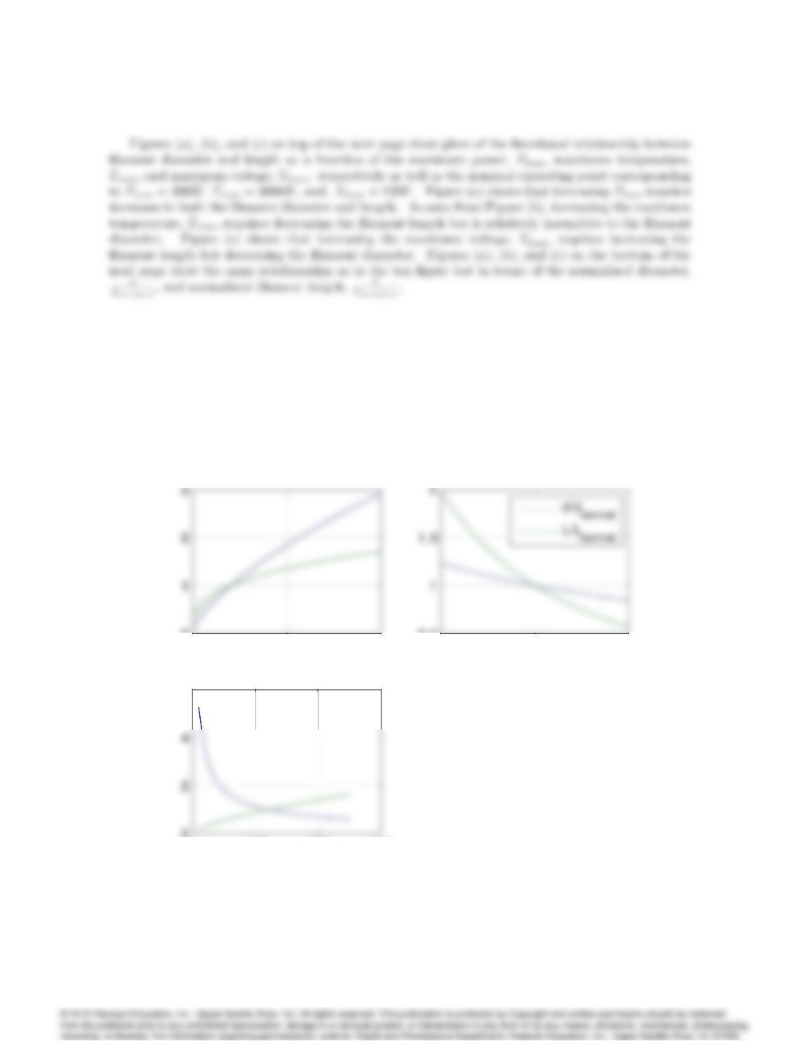
(2), in the steady-state, _

T= 0;and with V= 1,

and we can solve Eqs. (2) and (3), for d and L as follows. Equation (3) can be written as,

where,

are prescribed. Then, the filament diameter, d, is simply related to filament length, L, by,

Using Eq. (8) together with Eqs. (5) and (6), we can then solve for the filament length , L, as,

This can be simplified further by assuming that the maximum filament temperature is much higher

than the ambient temperature, T4

max T4

1;so that,

10074 CHAPTER 10. CONTROL-SYSTEM DESIGN: PRINCIPLES AND CASE STUDIES

0500 1000

0

(a) Pmax

0100 200 300

0

6

(b) Vmax(V)

2000 2500 3000

0.5

(c) T m ax(K)

0500 1000

0

(a) Pmax

d [mm]L [m]

0500 1000

0

(a) Pmax

0100 200 300

0

6

(b) Vmax(V)

d [mm]L [m]

0500 1000

0

(a) Pmax

d [mm]L [m]

0500 1000

0

(a) Pmax

0100 200 300

0

6

(b) Vmax(V)

2000 2500 3000

0.5

(c) T m ax(K)

0500 1000

0

(a) Pmax

d [mm]L [m]

0500 1000

0

(a) Pmax

0100 200 300

0

6

(b) Vmax(V)

d [mm]L [m]

0500 1000

0

(a) Pmax

d [mm]L [m]

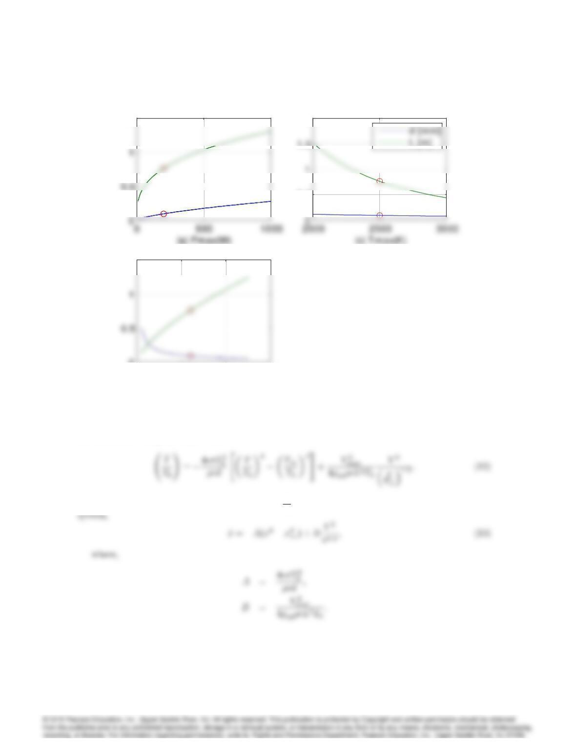
Problem 10.20: Lamp design parametrs.

10075

1.5

0100 200 300

0

1.5

(b) Vmax(V)

1.5

0100 200 300

0

1.5

(b) Vmax(V)

0.5

1.5

2

1.5

0100 200 300

0

1.5

(b) Vmax(V)

1.5

0100 200 300

0

1.5

(b) Vmax(V)

0.5

1.5

2

Problem 10.21: Lamp design parameters: normalized.

Assume the nominal operating temperature is denoted by T0. Re-writing Equation (2) in terms of

the normalized temperature, we have

Let us define the normalized temperature, x=T

T0;and re-write Eq. (12) as the nonlinear first-order

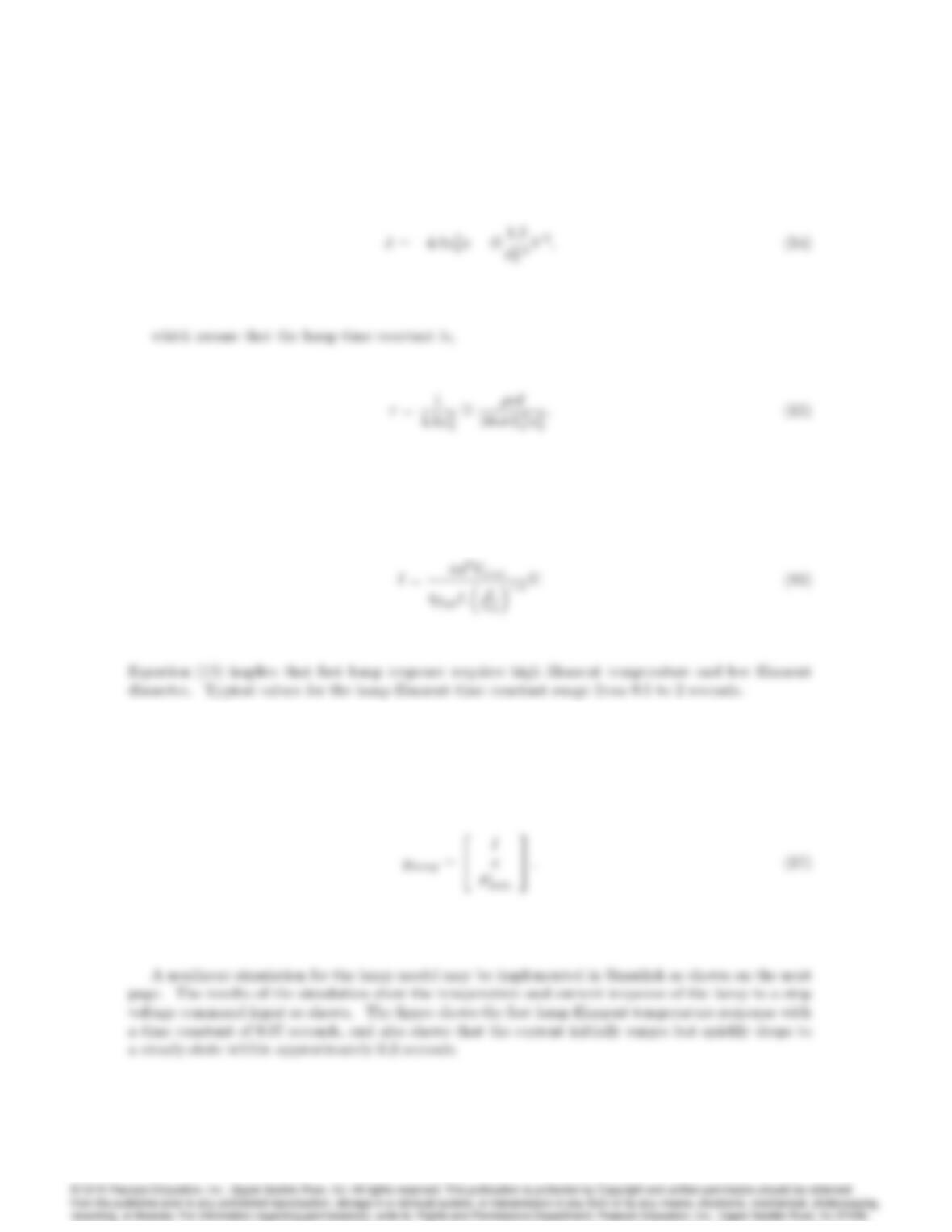
Linearizing Equation (13) about the nominal (normalized) temperature, we find the first-order

10076 CHAPTER 10. CONTROL-SYSTEM DESIGN: PRINCIPLES AND CASE STUDIES

linear dynamic model for the lamp as,

In terms of lamp current, we have,

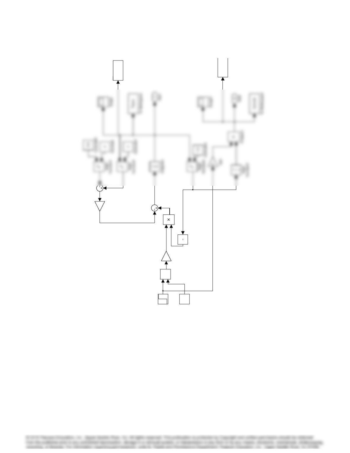
The output of the lamp may be considered to be current, normalized filament temperature, or

radiative power,

10077

I current . mat

To File1

ToT. m at

To File

Step

Product

1

u

Math

Function4

uv

Math

Funct ion

b

Gain2

a

Gain1

2

Cons tant 3

Problem 10.21: Simulink diagram for lamp model.

10078 CHAPTER 10. CONTROL-SYSTEM DESIGN: PRINCIPLES AND CASE STUDIES

00.1 0.2 0.3 0.4 0.5

0

2

4

6

8

10

12

14

Time (sec)

Filament temperature, current

Response to step voltage command

00.1 0.2 0.3 0.4 0.5

0

2

4

6

8

10

12

14

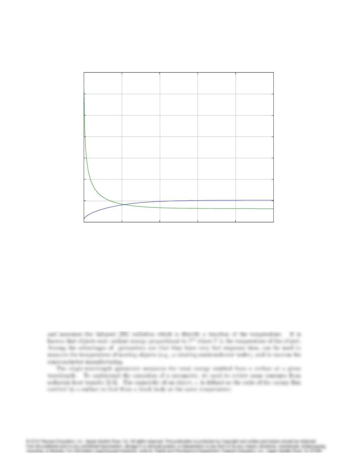
Problem 10.21: Lamp response to a step voltage command.

References:

[1] Reynolds, W. C., and H. C. Perkins, Engineering Thermodynamics, McGraw-Hill, 1977.

[2] A. Emami-Naeini, et al., “Modeling and Control of Distributed Thermal Systems,” IEEE Tran.

Contrl. Syst. Tech., pp. 668-683, September 2003.

[3] Lide, D. R., Ed., Handbook of Chemistry and Physics, CRC Press, 1993-1994.

[4] Modest, M. F., Radiative Heat Transfer, McGraw-Hill, 1993.

23. Develop a nonlinear model for a pyrometer. Show how temperature can be deduced from the

model.

Solution:

Temperature measurement can be done by a variety of methods including thermocouples, resistive

temperature detectors (RTDs), and pyrometers [1]. A pyrometer is a non-contact temperature sensor

where,

=total emissivity,

=spectral emissivity,

where,

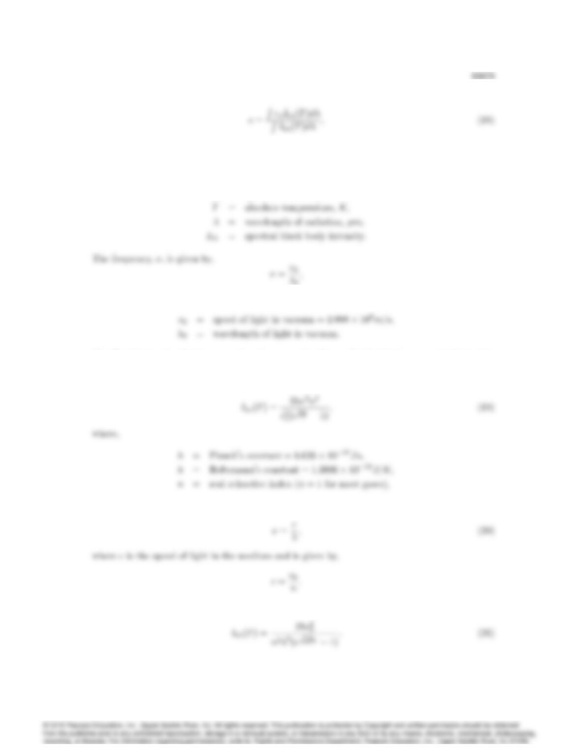
The Plank’s law of radiation states that the spectral radiance of a blackbody, or spectral intensity,

Ib , in a dielectric medium as a function of the wavelength and temperature is,

and the frequency and wavelength are related by,

After some manipulation, we can re-write Eq. (19) as [2],