
Solutions Manual&KDSWHU
7th Edition
Feedback Control of Dynamic
Systems
Gene F. Franklin
J. David Powell
Abbas Emami-Naeini .
Assisted by:
H.K. Aghajan
H. Al-Rahmani
P. Coulot
P. Dankoski
S. Everett
R. Fuller
T. Iwata
V. Jones
F. Safai
L. Kobayashi
H-T. Lee
E. Thuriyasena
M. Matsuoka
J.K. Lee
1
h t 1
ont o t i n in i
nd t di
Problems and Solutions for Cha ter 1
1. f the three t es of PID control or integra or derivativ which one is the most
ective in reducing the error resulting from a constant disturbance lain.
Integral control is the most e ective in reducing the error due to constant disturbances.
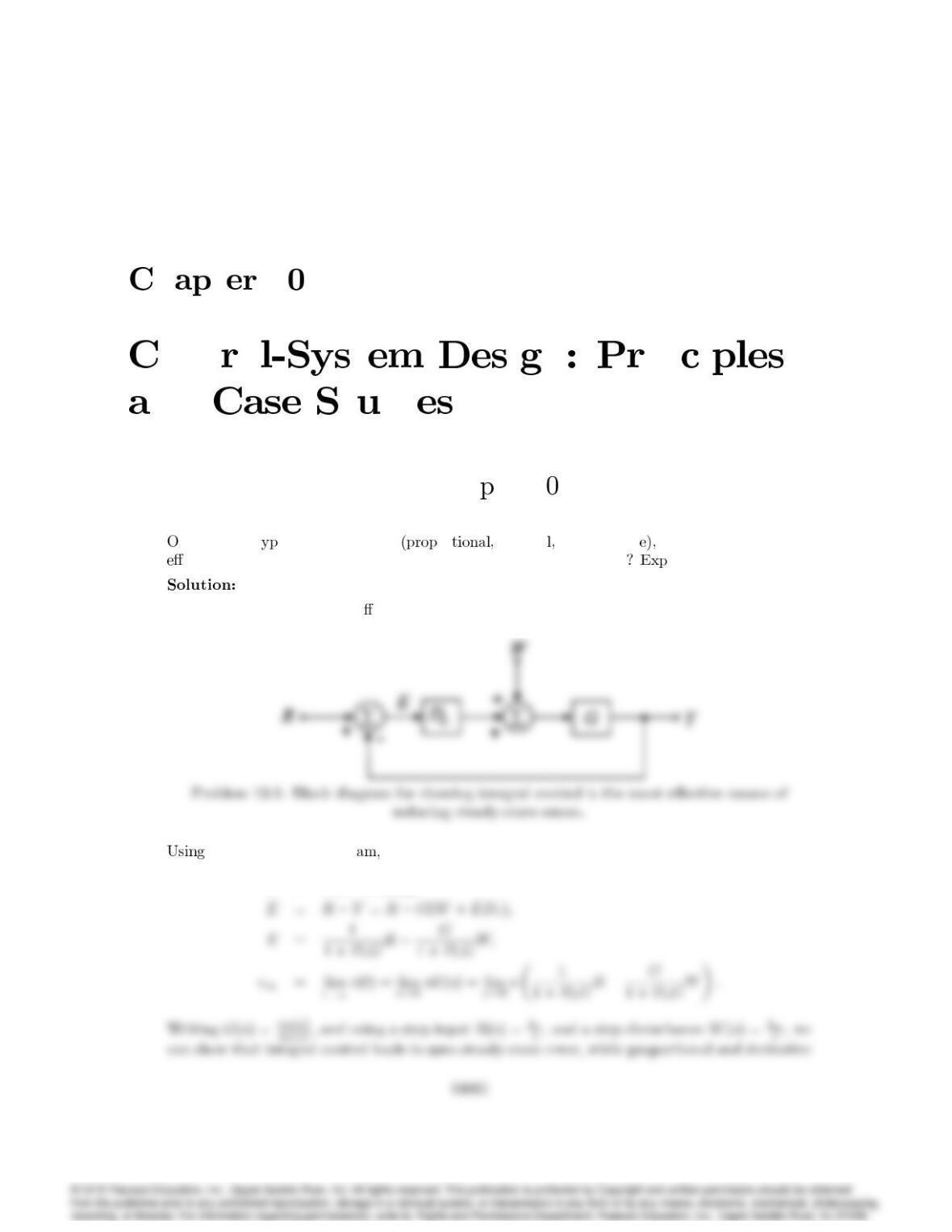
the above block diagr
Y=G(W+EDc);
CHAPTER 10. CONTROL-SYSTEM DESIGN: PRINCIPLES AND CASE STUDIES
contr in gener do not.
Is there a greater chance of instability when the sensor in a feedback control system for a
mechanical structure is not collocated with the actuator n.
Solution:
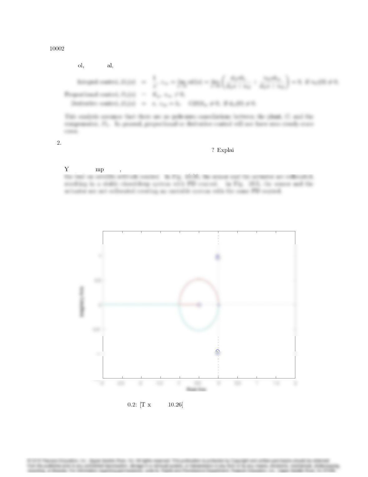
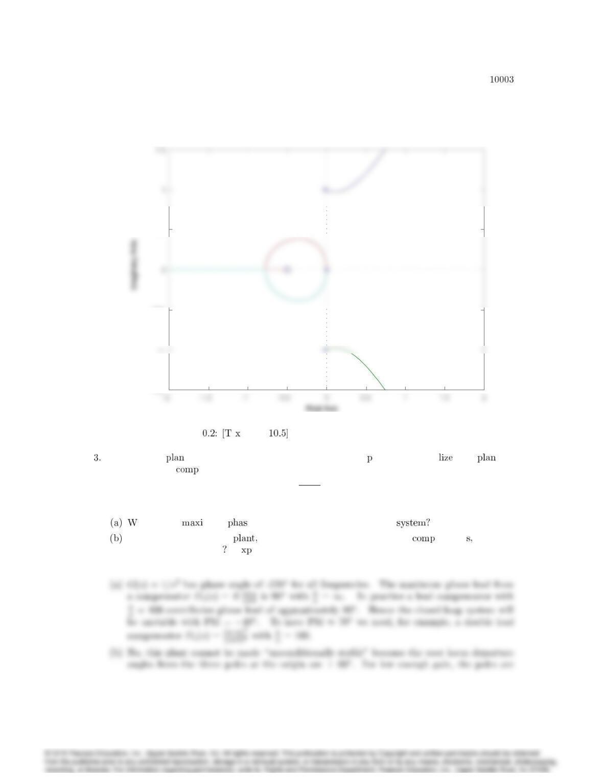
es. For co arison see the following two root loci which were taken from the discussion in
1.5
Root Locus
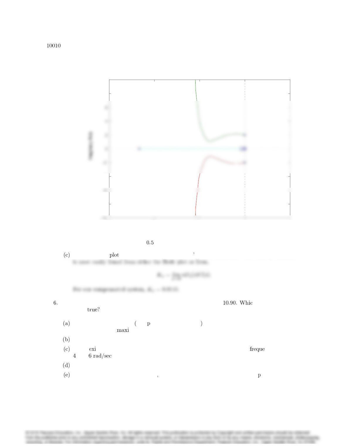
Problem 1 e t Fig. PD control of satellite: collocated.
–0.5
0.5
Root Locus
Problem 1 e t Fig. PD control of satellite: non-collocated.
Consider the t G(s) = 1=s3. Determine whether it is ossible to stabi this t by
adding the lead ensator
Dc(s) = Ks+a
s+b;(a < b):
hat is the mum e margin of the resulting feedback
Can a system with this together with any number of lead ensator be made
unconditionally stable E lain why or why not.
Solution:
CHAPTER 10. CONTROL-SYSTEM DESIGN: PRINCIPLES AND CASE STUDIES
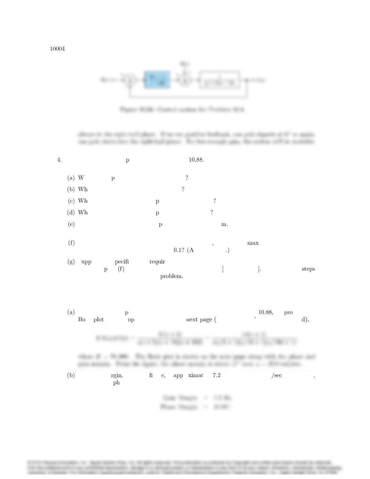
Consider the closed-loo system shown in Fig.
hat is the hase margin if K= 70;000
at is the gain margin if K= 70;000
at value of Kwill yield a hase margin of 70
at value of Kwill yield a hase margin of 0
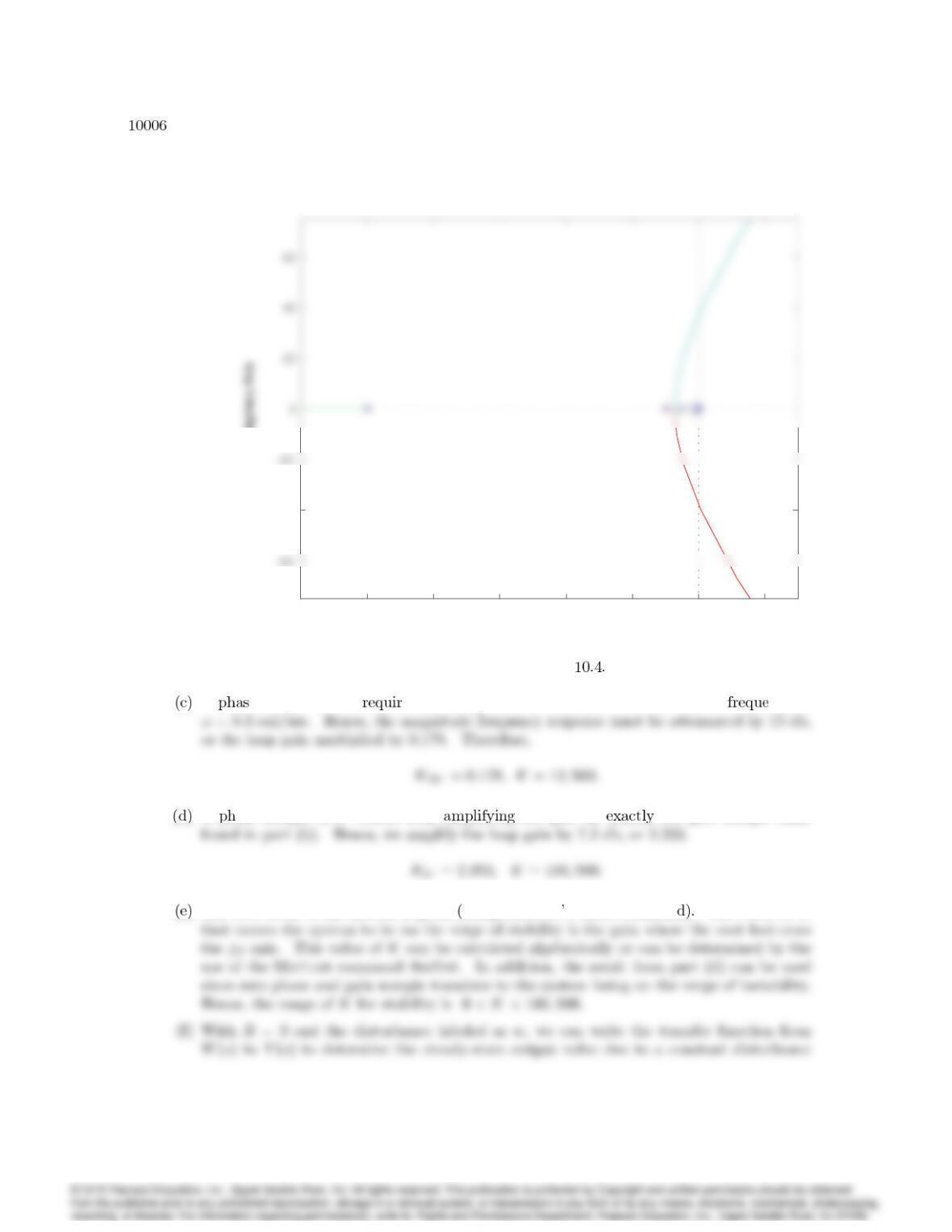
Sketch the root locus with res ect to Kfor the syste and determine what value of K
causes the system to be on the verge of instability.
If the disturbance wis a constant and K= 10;000 what is the imum allowable value
for wif y(1)is to remain less than ssume r= 0
S ose the s cations e you to allow larger values of wthan the value you ob-
tained in art but with the same error constraint jy(1)j<0:1Discuss what
you could take to alleviate the
Solution:
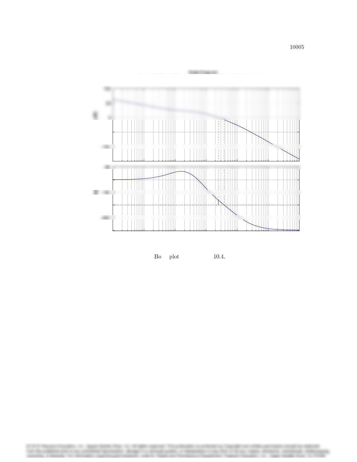
To determine the hase and gain margin of the system given in Fig. we duce the
de of the lo gain shown on the using Matlab smargin comman
The gain ma from the gur is ro ely db at != 38:0rad . Therefore
the gain and ase margins are
–150
–50
Magnitude (dB)
10
-2
10
-1
10
0
10
1
10
2
10
3
10
4
–270
–180
–90
Phase ( deg)
Gm = 7.2 dB (at 37.9 rad/sec) , Pm = 17 deg (at 24.9 rad/sec)
Freq uency (r ad/sec)
–150
–50
Magnitude (dB)
10
-2
10
-1
10
0
10
1
10
2
10
3
10
4
–270
–180
–90
Phase ( deg)
de for Problem
CHAPTER 10. CONTROL-SYSTEM DESIGN: PRINCIPLES AND CASE STUDIES
–120 – 100 – 80 –60 – 40 –20 020
–40
Root Locus
Real Axis
Imaginar y Axis
Root Locus for Problem
A e margin of 70es the magnitude to cross the 0db line near a ncy of
A ase margin of 0results from the gain by the gain margin value
The root locus of the system is given using Matlab srlocus comman The value of K
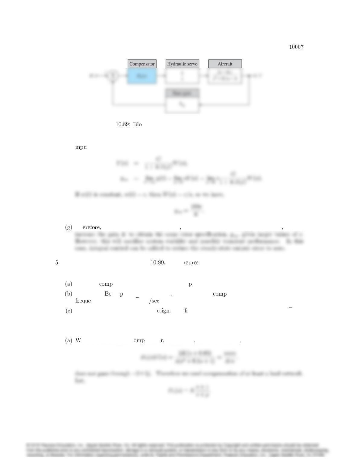
Figure ck diagram for aircraft-attitude rate control.
t.
Th with K= 10000 and y < 0:1we have c < 10. Since yss = 100c=K we can
Consider the system shown in Fig. which ents the attitude rate control for a certain
aircraft.
Design a ensator so that the dominant oles are at 22j.
Sketch the de lot for your design and select the ensation so that the crossover
ncy is at least 2p2rad and PM 50.
Sketch the root locus for your d and nd the velocity constant when !n>2p2and
0:5.
Solution:
ith a constant gain c ensato Dc(s) = Kthe root locus of

CHAPTER 10. CONTROL-SYSTEM DESIGN: PRINCIPLES AND CASE STUDIES
the angle criter at the closed-lo ole location s=2 + 2jwe can write an
sion for the angle contribution from the lead network zand lead network
p.
So we hav =zp= 117. In Matlab
selection of z= 0:4we get p= 11:7. So that our lead design is
To nd the ensator gain Kwe can utili e the magnitude criterion at the desired
dominant closed-lo ole locations. e nd
So the lead design
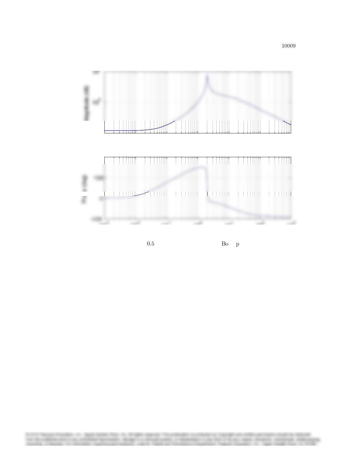
The de of the system lo transfer funct
10-3 10-2 10-1 100101102103
10-2
Magnitude (dB)
10-3 10-2 10-1 100101102103
10-2
Magnitude (dB)
10-3 10-2 10-1 100101102103
200
phase
Frequency (rad/sec)
10-3 10-2 10-1 100101102103
10-2
Magnitude (dB)
10-3 10-2 10-1 100101102103
10-2
Magnitude (dB)
10-3 10-2 10-1 100101102103
200
phase
Frequency (rad/sec)
Problem 1 PD control of an aircraft: de lot.
CHAPTER 10. CONTROL-SYSTEM DESIGN: PRINCIPLES AND CASE STUDIES
–15 – 10 -5 0 5
-8
-4
8
10
Root Locus
Real Axis
Problem 1 PD control of an aircraft: root locus.
The root locus is shown above using Matlab srlocus command. The velocity constant
Consider the block diagram for the servomechanism drawn in Fig. h of the following
claims are
The actuator dynamics the ole at 1000 rad=sec must be included in an analysis to
evaluate a usable mum gain for which the control system is stable.
The gain Kmust be negative for the system to be stable.
There sts a value of Kfor which the control system will oscillate at a ncy between
and .
The system is unstable if jKj>10.
If Kmust be negative for stability the control system cannot counteract a ositive distur-
bance.
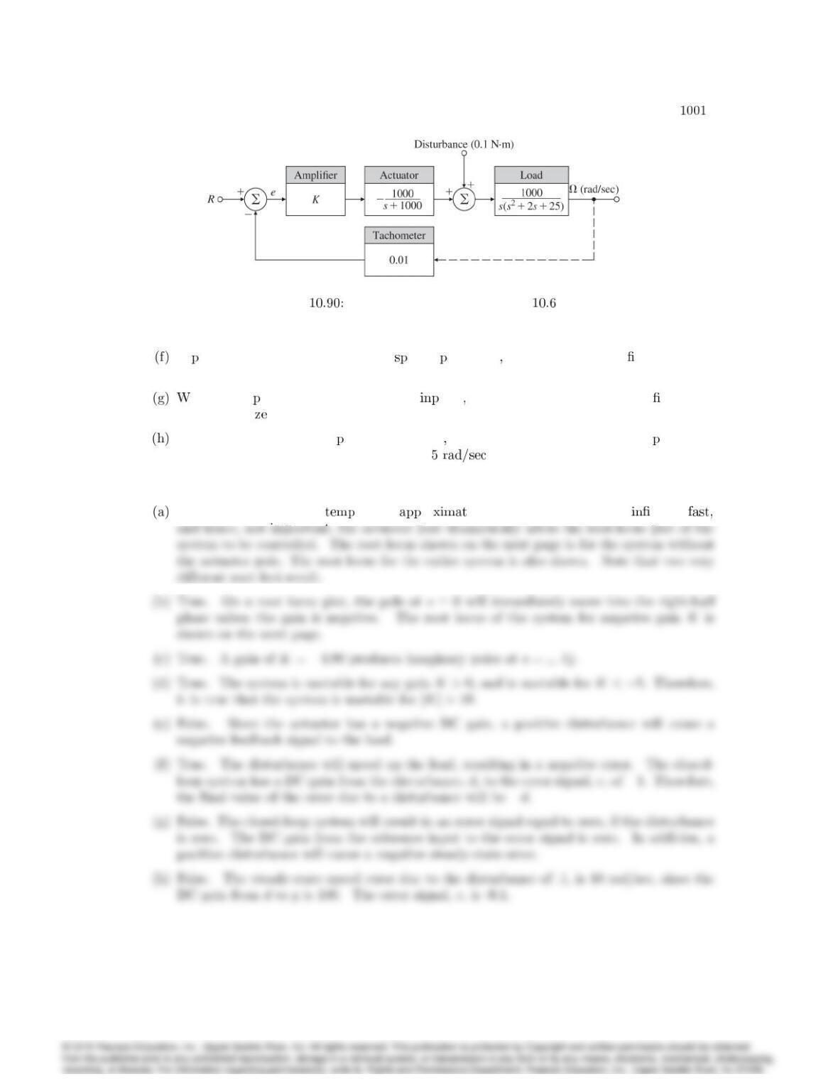
1
Figure Servomechanism for Problem. .
A ositive constant disturbance will eed u the load thereby making the nal value of e
negative.
ith only a ositive constant command ut rthe error signal emust have a nal value
greater than ro.
For K=1the closed-loo system is stable and the disturbance results in a s eed error
whose steady-state magnitude is less than .
Solution:
True. Even though it is ting to ro e the actuator dynamics as nitely
CHAPTER 10. CONTROL-SYSTEM DESIGN: PRINCIPLES AND CASE STUDIES
–10 -8 -6 -4 -2 0 2 4 6 8 10
-8
-2
0
10
Root Locus
Real Axis
Imaginar y Axis
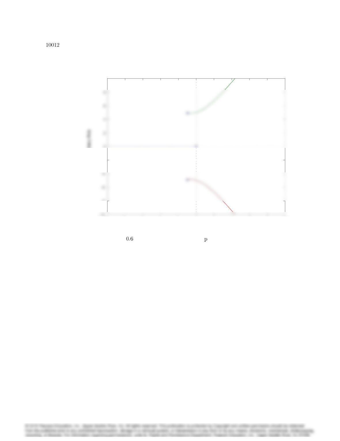
Problem 1 Servo mechanical root locus lot: without actuator.
–10 -8 -6 -4 -2 0 2 4 6 8 10
-8
-2
8
10
Root Locus
Real Axis
Imaginar y Axis
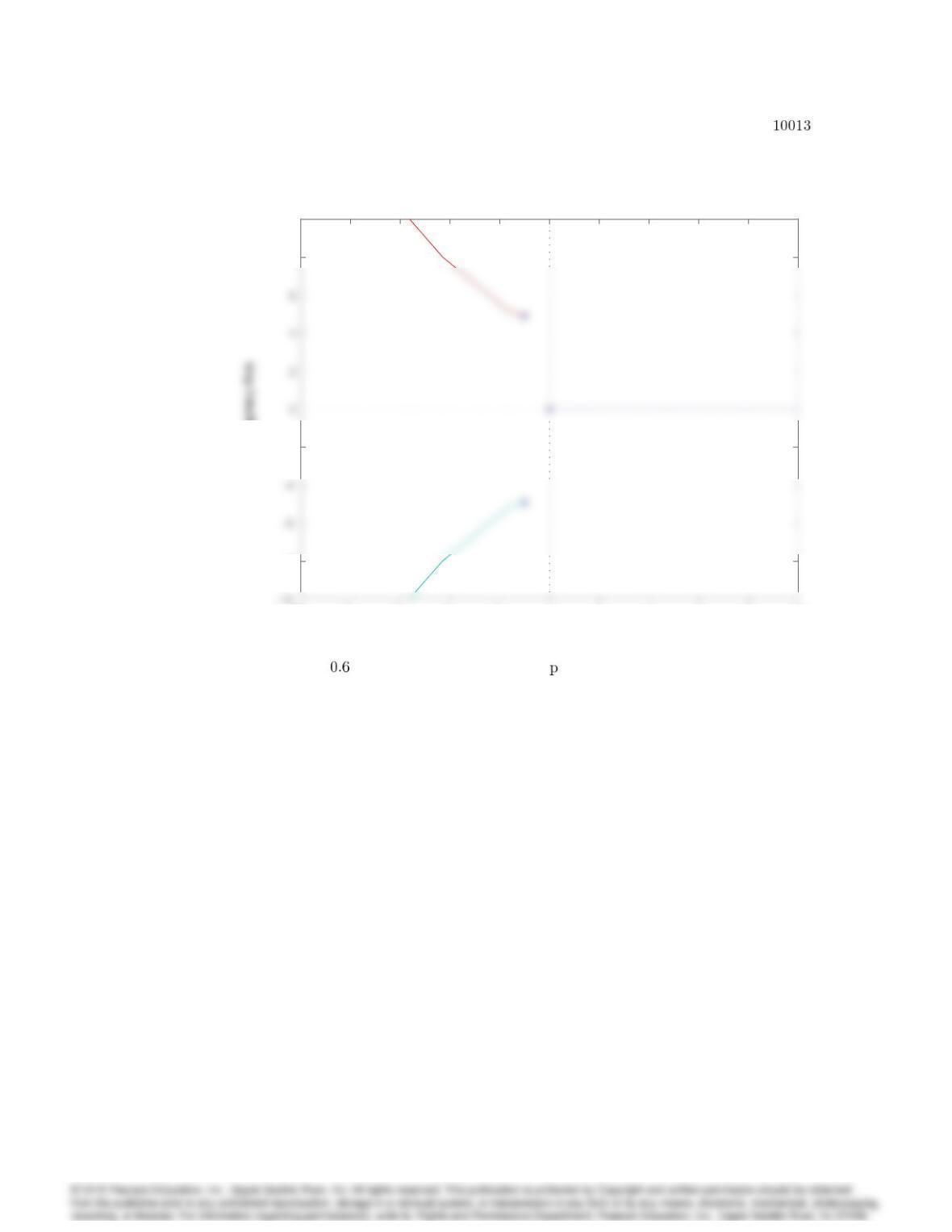
Problem 1 Servo mechanical root locus lot: with actuator dynamics.
CHAPTER 10. CONTROL-SYSTEM DESIGN: PRINCIPLES AND CASE STUDIES
–10 -8 -6 -4 -2 0 2 4 6 8 10
-8
-2
8
10
Root Locus
Real Axis
Imaginar y Axis
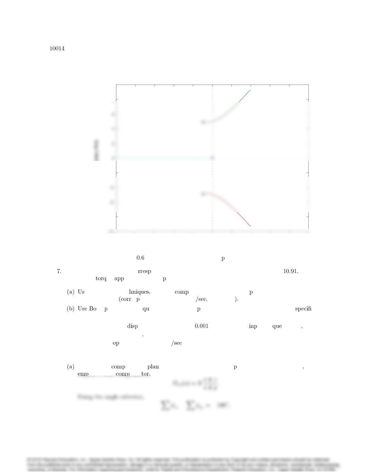
Problem 1 Servo mechanical root locus lot: for negative gain.
A stick balancer and its co onding control block diagram are shown in Fig. The
control is a ue lied about the ivot.
ing root-locus tec design a ensator Dc(s)that will lace the dominant roots
at s=55jes onding to !n= 7 rad = 0:707
de lotting techni es to design a com ensator Dc(s)to meet the following –
cations:
steady-state lacement of less than for a constant ut tor Td= 1
Phase Margin 50
Closed-lo bandwidth
=7rad .
Solution:
To have the ensated t root locus go through the ole location s=55jwe
or
In Matlab
To nd the ensator gain Kwe can utili e the magnitude criterion at the desired
dominant closed-lo ole locations. e nd
CHAPTER 10. CONTROL-SYSTEM DESIGN: PRINCIPLES AND CASE STUDIES
–60 – 50 –40 – 30 –20 –10 010 20
–20
Root Locus
Real Axis
Imaginar y Axis
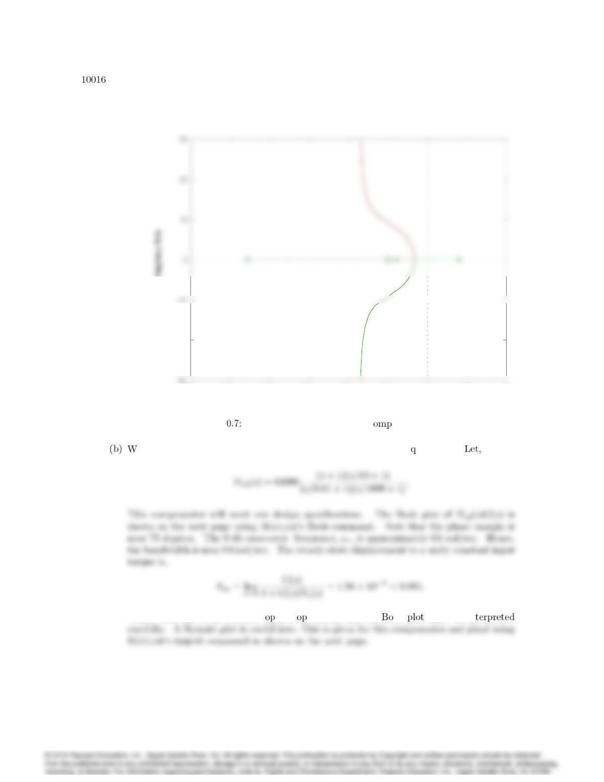
Problem 1 Root locus of stick balancer c ensated system.
e need a lag network in addition to a lead network to get the re uired Kp.
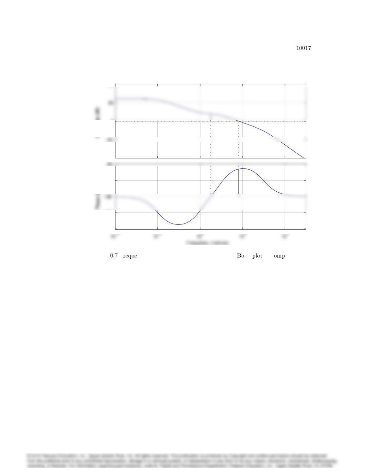
Notice that this is an unstable en-lo system and the de must be in
–100
0
100
–270
–225
–135
Bode Diag ram
Gm = –19.6 dB (at 3.16 rad/sec) , Pm = 76.5 deg (at 63.7 rad/sec)
–100
0
100
–270
–225
–135
Problem 1 F ncy design method for stick balancer: de of c ensated
system.
CHAPTER 10. CONTROL-SYSTEM DESIGN: PRINCIPLES AND CASE STUDIES
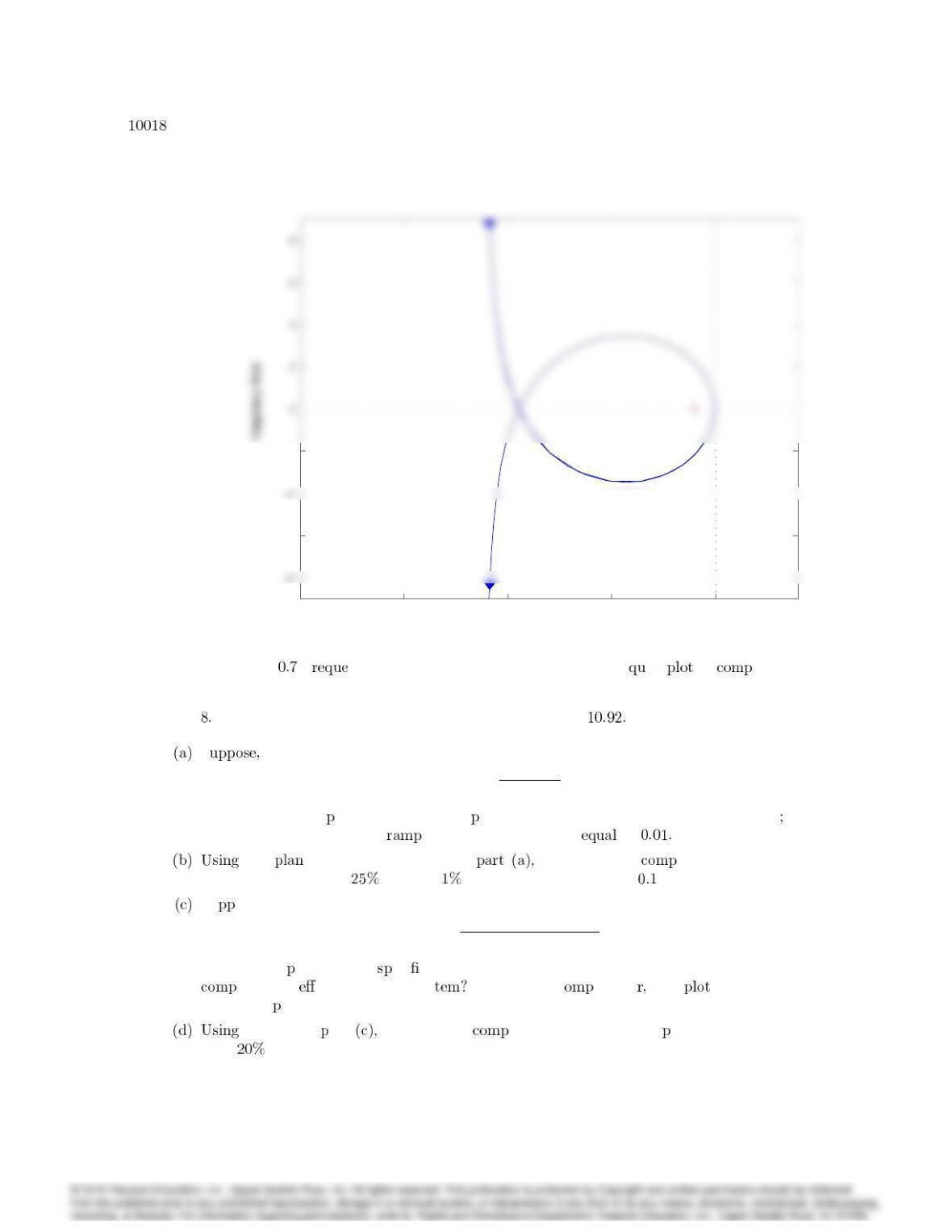
–20 –15 – 10 -5 0
-6
-2
Nyq uist Diag ram
Real Axis
Problem 1 F ncy design method for stick balancer: Ny ist of ensated
system.
Consider the standard feedback system drawn in Fig.
S
G(s) = 2500 K
s(s+ 25):
Design a lead com ensator so that the hase margin of the system is more than 45the
steady-state error due to a should be less than or to
the t transfer function from design a lead ensator so that the
overshoot is less than and the settling time is less than sec.
Su ose
G(s) = K
s(1 + 0:1s)(1 + 0:2s);
and let the erformance eci cations now be Kv= 100 and PM 40. Is the lead
ensation ective for this sys Find a lag c ensato and the root locus
of the com ensated system.
G(s)from art design a lag ensator such that the eak overshoot is less
than and Kv= 100.
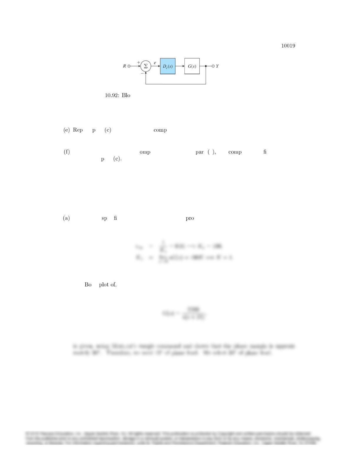
Figure ck diagram of a standard feedback control system.
eat art using a lead-lag ensator.
Find the root locus of the c ensated system in t e and are your ndings with
those from art
Solution:
The design eci cation of steady-state error vides information for the design of K.
The de