10020 CHAPTER 10. CONTROL-SYSTEM DESIGN: PRINCIPLES AND CASE STUDIES
–40
Phase (deg)
Bode D iag ram
Frequency (rad/sec)
–40
Phase (deg)
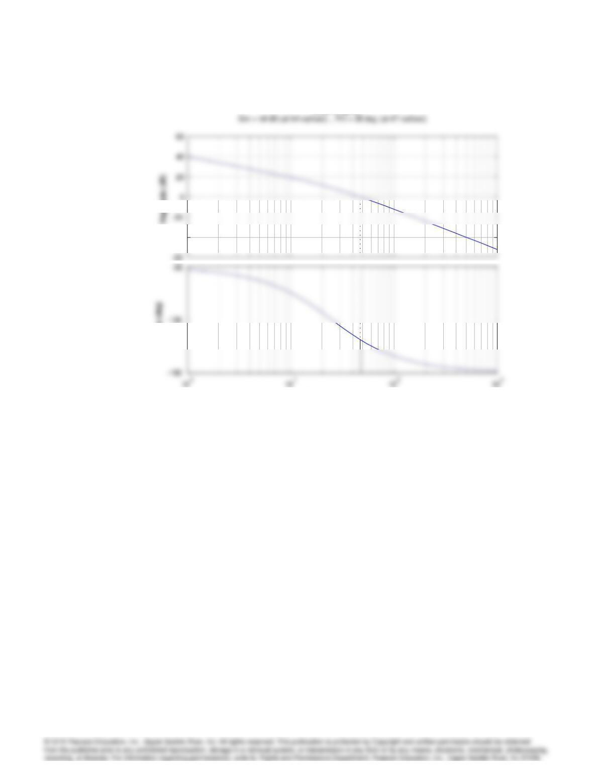
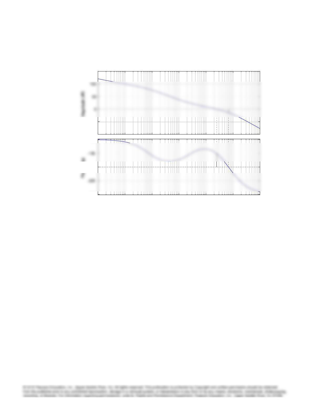
Problem 10.8: Frequency response of G(s).
10021
50
Magnitude ( dB)
10
0
10
1
10
2
10
3
10
4
–180
–90
Phase (deg)
Bode D iag ram
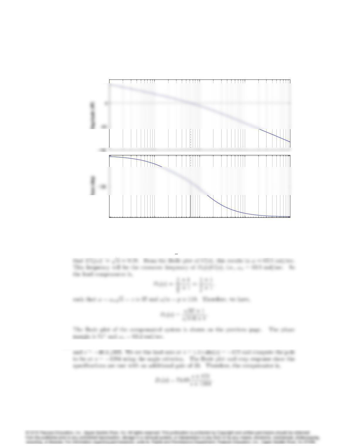
Gm = Inf dB (at Inf rad/sec) , Pm = 51.4 deg (at 63.1 rad/sec)
Frequency (r ad/sec)
50
Magnitude (dB)
10
0
10
1
10
2
10
3
10
4
–180
–90
Phase (deg)
Problem 10.8: Frequency response of Dc(s)G(s).
From text Fig. 6.53 of the text, we have 1
= 3. Now, we need to find the frequency such
(b) For Mp= 25%, let = 0:4. For ts<0:1, let !nt4:6=0:1 = 46. Thus, !n= 115 rad/sec,
10022 CHAPTER 10. CONTROL-SYSTEM DESIGN: PRINCIPLES AND CASE STUDIES
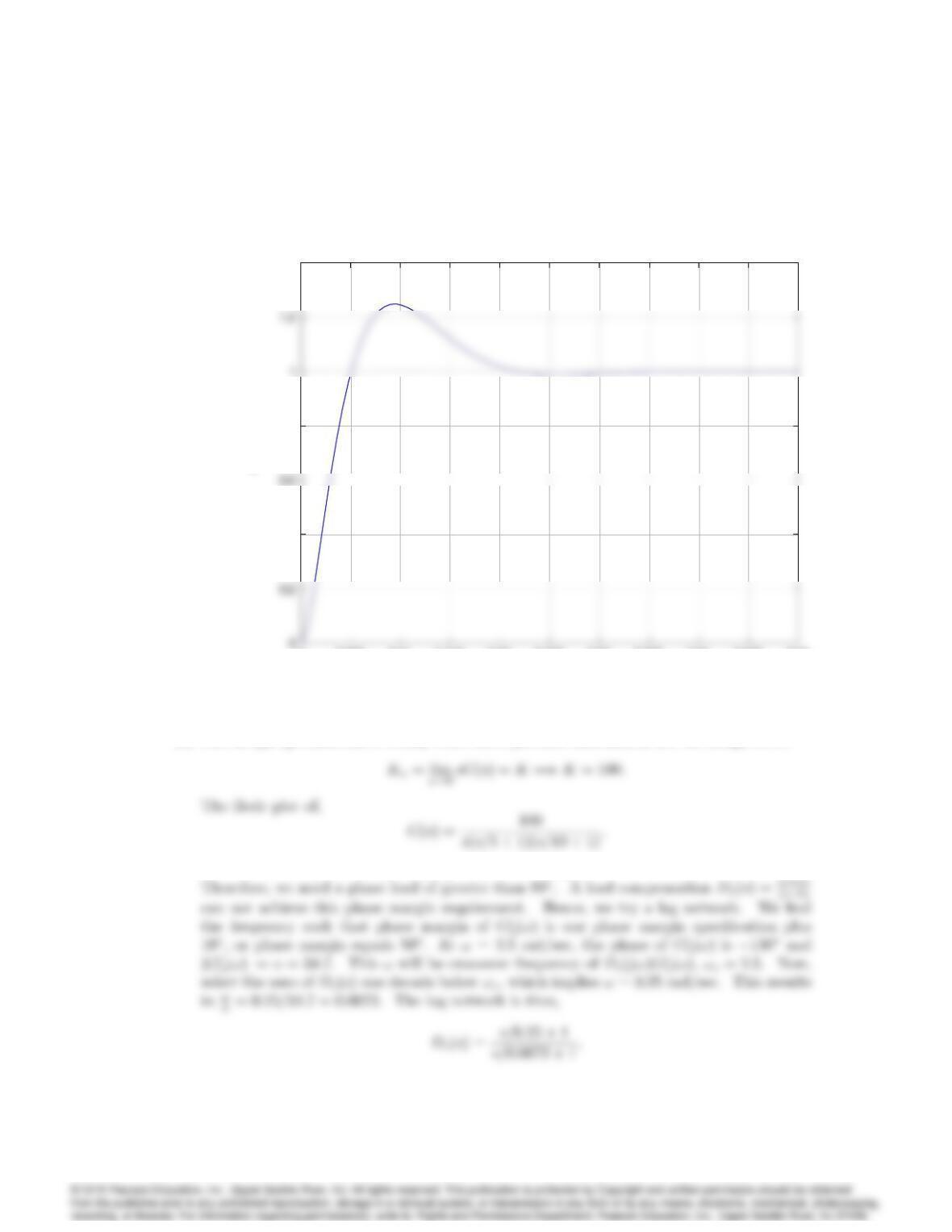
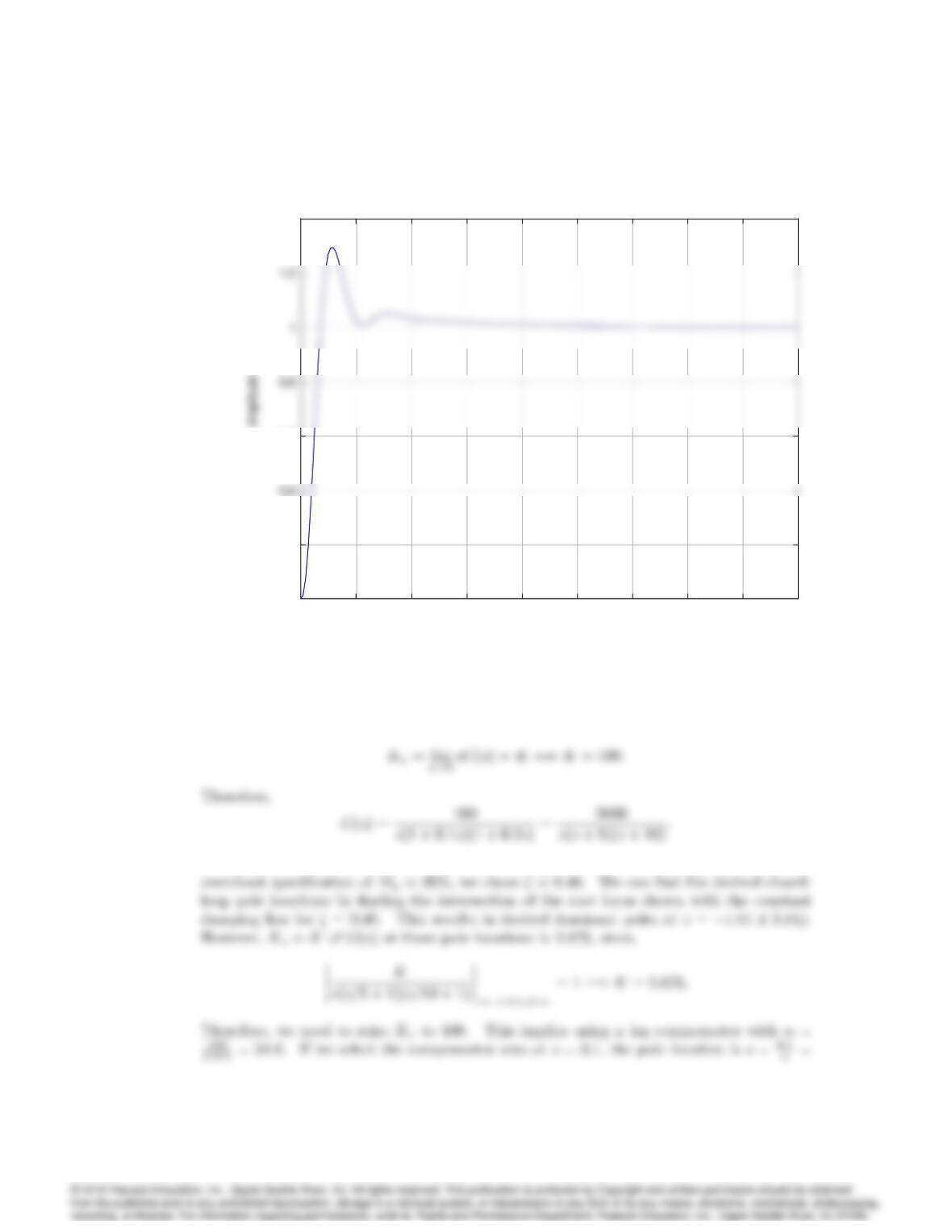
The closed-loop step response is shown below (using Matlab’s step command).
00.005 0.01 0.015 0.02 0.025 0.03 0.035 0.04 0.045 0.05
0.4
0.8
1.4
Step R esponse
Time (sec)
Amplitude
00.005 0.01 0.015 0.02 0.025 0.03 0.035 0.04 0.045 0.05
0.4
0.8
1.4
Step response of the closed-loop system for Problem 10.8 (b).
(c) The design specification of steady-state error provides information for the design of K.
shows that the phase margin (using Matlab’s margin) is 40:This is shown below.
10023
and the loop gain is,
–60
–40
–20
Magnitude (dB)
10
-1
10
0
10
1
10
2
–270
–225
–180
Phase (deg)
–60
–40
–20
Magnitude (dB)
10
-1
10
0
10
1
10
2
–270
–225
–180
Phase (deg)
10024 CHAPTER 10. CONTROL-SYSTEM DESIGN: PRINCIPLES AND CASE STUDIES
–100
–50
150
10
-4
10
-3
10
-2
10
-1
10
0
10
1
10
2
–270
–180
–90
Bode D iag ram
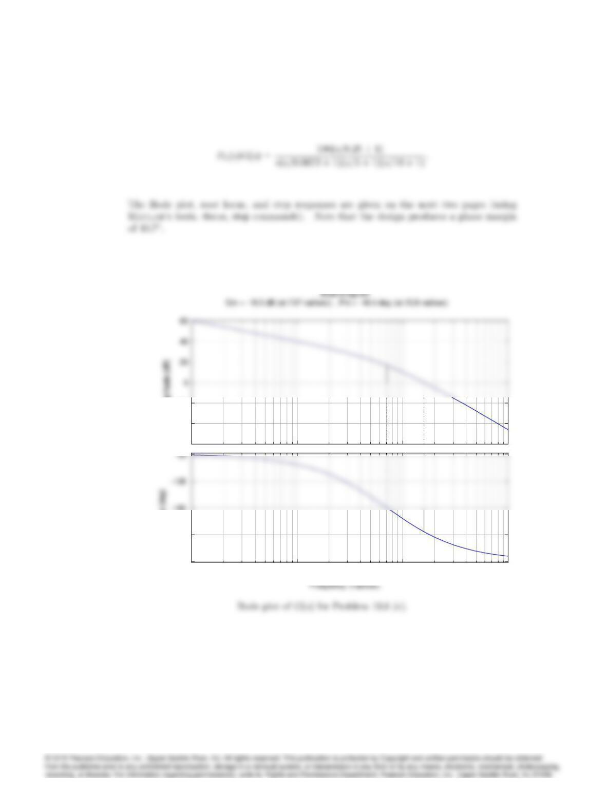
Gm = 13.7 dB (at 6.81 rad/sec) , Pm = 43.7 deg (at 2.51 rad/sec)
Frequency (r ad/sec)
–100
–50
150
10
-4
10
-3
10
-2
10
-1
10
0
10
1
10
2
–270
–180
–90
Bode plot of Dc(s)G(s)for Problem 10.8 (c).
10025
–12 –10 -8 -6 -4 -2 0 2 4
-1
3
4
Root Locus
Real Axis
Imaginar y Axis
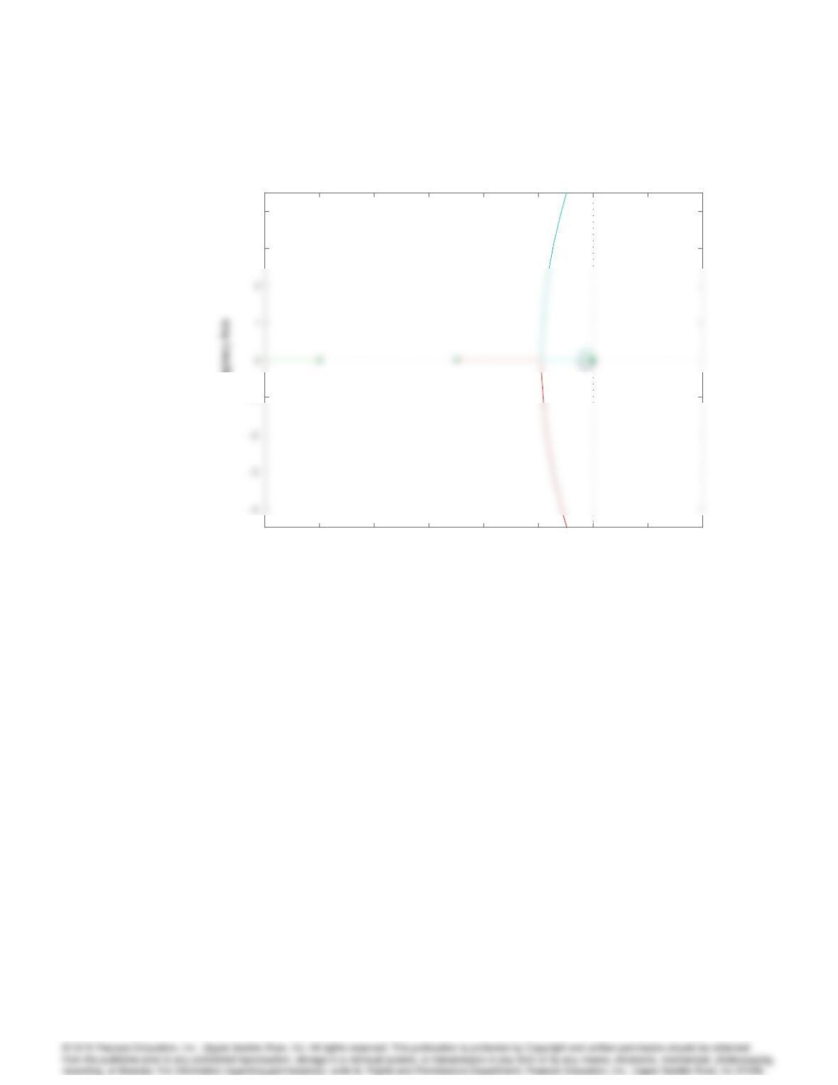
Root locus of Dc(s)G(s)for Problem 10.8 (c).
10026 CHAPTER 10. CONTROL-SYSTEM DESIGN: PRINCIPLES AND CASE STUDIES
0 2 4 6 8 10 12 14 16 18
0
0.2
0.6
1.4
Step R esponse
Time (sec)
0 2 4 6 8 10 12 14 16 18
0
0.2
0.6
1.4
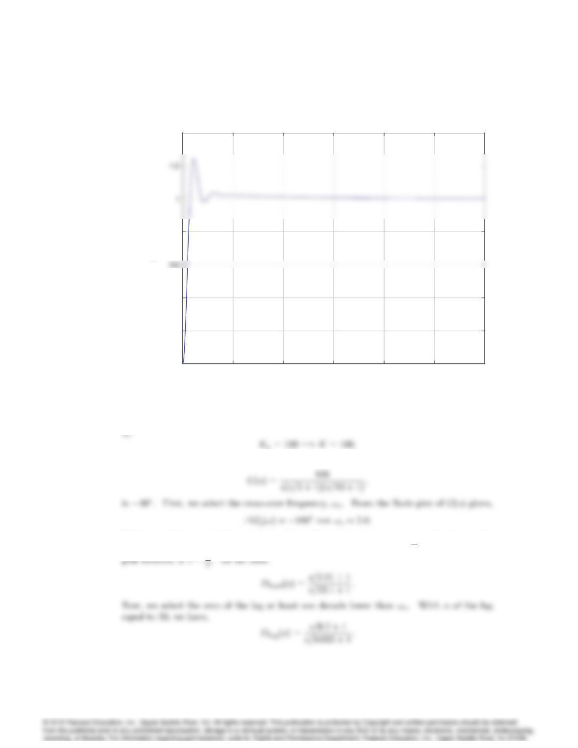
Step response of closed-loop system for Problem 10.8 (c).
(d) We can design a lag compensator using root locus methods. The velocity constant requires
the plant gain to be equal to 100, since,
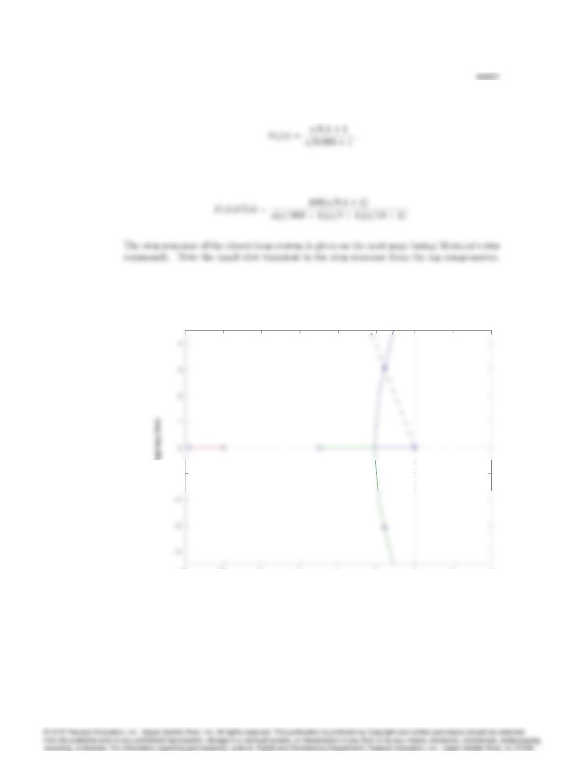
The root locus plot of G(s)is shown below using Matlab’s rlocus command. For an
0:003. Hence,
and the loop gain is,
–12 –10 -8 -6 -4 -2 0 2 4
-1
Root Locus
Real Axis
Imaginar y Axis
Root locus for Problem 10.8 (d).
10028 CHAPTER 10. CONTROL-SYSTEM DESIGN: PRINCIPLES AND CASE STUDIES
0 5 10 15 20 25 30
0
0.2
0.4
0.8
1.4
Step R esponse
Time (sec)
Amplitude
0 5 10 15 20 25 30
0
0.2
0.4
0.8
1.4
Step response of closed-loop system for Problem 10.8 (d).
(e) Again, the design specification of steady-state error provides information for the design of
As mentioned in part (c), the phase margin for,
With !c= 7:0we need 40more lead. From Fig. 6.52 in the text, an = 0:1will provide
55of lead. We select the lead such that zero location is s=!=!cp= 2:21. The lead
10029
The lead-lag compensator is,
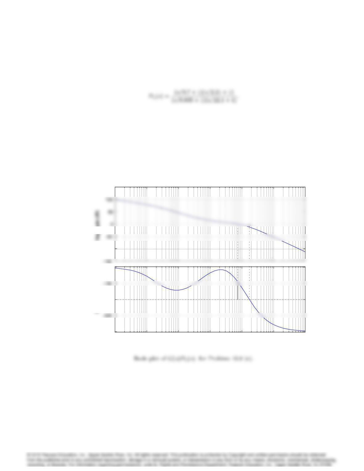
The system Bode plot and step response appear on the next page.
–100
150
10
-3
10
-2
10
-1
10
0
10
1
10
2
10
3
–270
–180
–90
Bode D iag ram
Gm = 11.9 dB (at 17.2 rad/sec) , Pm = 49.1 deg (at 7.45 rad/sec)
Frequency (r ad/sec)
–100
150
10
-3
10
-2
10
-1
10
0
10
1
10
2
10
3
–270
–180
–90
10030 CHAPTER 10. CONTROL-SYSTEM DESIGN: PRINCIPLES AND CASE STUDIES
0 1 2 3 4 5 6
0
0.2
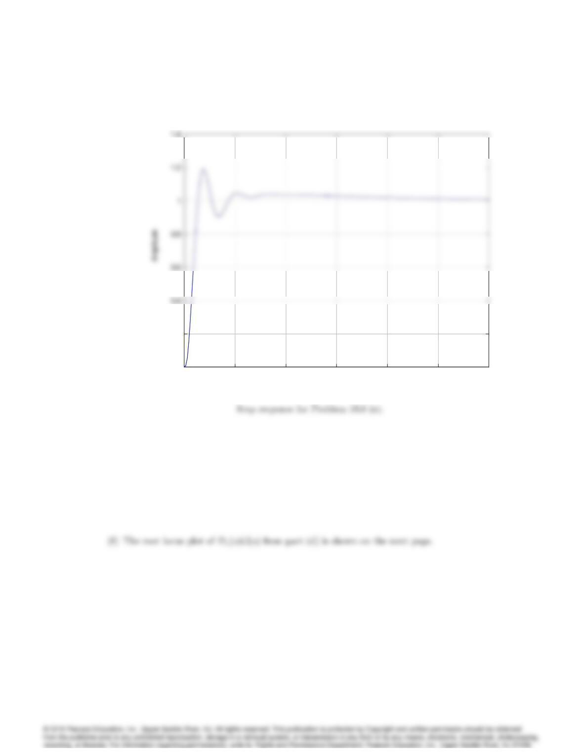
Step r esponse for the lead- lag design of Problem 10.8(e)
Time (sec)
0 1 2 3 4 5 6
0
0.2
10031
–12 –10 -8 -6 -4 -2 0 2 4
-3
-1
4
Root Locus
Real Axis
Imaginar y Axis
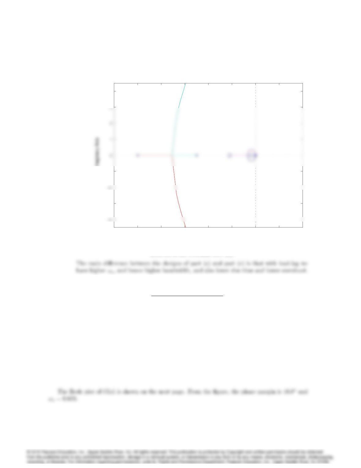
Root locus for Problem 10.8 (e).
9. Consider the system in Fig. 10.92, where
G(s) = 300
s(s+ 0:225)(s+ 4)(s+ 180):
The compensator Dc(s)is to be designed so that the closed-loop system satisfies the following speci-
fications:
1. zero steady-state error for step inputs,
PM = 55,GM 6db,
gain crossover frequency is not smaller than that of the uncompensated plant.
(a) What kind of compensation should be used and why?
(b) Design a suitable compensator Dc(s)to meet the specifications.
Solution:
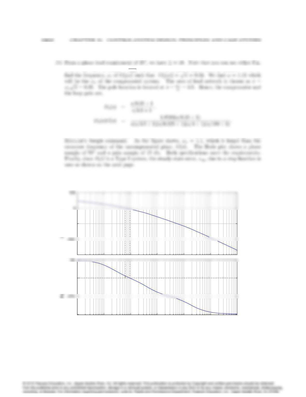
1. (a) Since we need 5510= 45of phase lead, a single lead network will do the job.
6.52 of the text, or sin() = 1
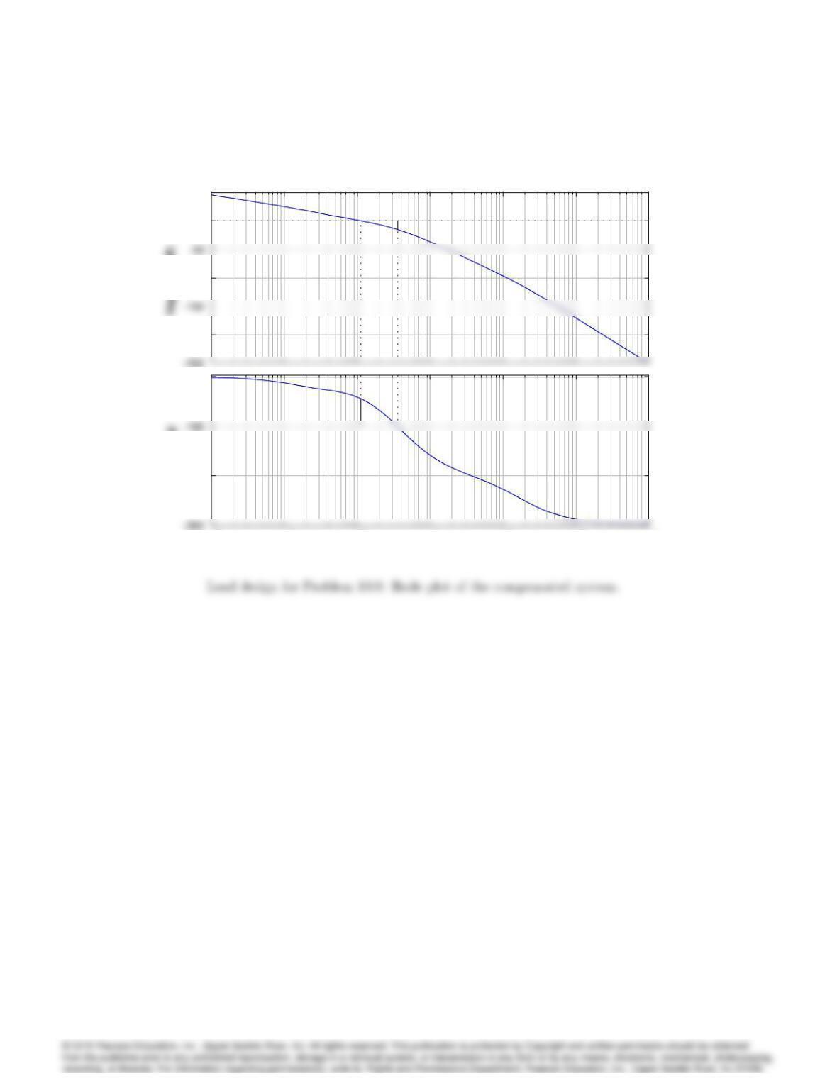
The Bode plot of Dc(s)G(s), the compensated system is shown on the next page using
–300
–100
10
-2
10
-1
10
0
10
1
10
2
10
3
10
4
–360
–180
Bode D iag ram
Gm = 6.96 dB (at 0.938 rad/sec) , Pm = 10.8 deg (at 0.622 rad/sec)
Frequency (r ad/sec)
–300
–100
10
-2
10
-1
10
0
10
1
10
2
10
3
10
4
–360
–180
Bode plot of G(s)for Problem 10.9.
10033
–200
–100
0
50
10
-2
10
-1
10
0
10
1
10
2
10
3
10
4
–270
–90
Phase (deg)
Bode D iag ram
Gm = 15 dB (at 3.54 rad/sec) , Pm = 50.2 deg (at 1.12 rad/sec)
Frequency (r ad/sec)
–200
–100
0
50
10
-2
10
-1
10
0
10
1
10
2
10
3
10
4
–270
–90
Phase (deg)
10034 CHAPTER 10. CONTROL-SYSTEM DESIGN: PRINCIPLES AND CASE STUDIES
0 2 4 6 8 10 12 14
0
0.4
0.8
1.4
Step R esponse
Time (sec)
Amplitude
0 2 4 6 8 10 12 14
0
0.4
0.8
1.4
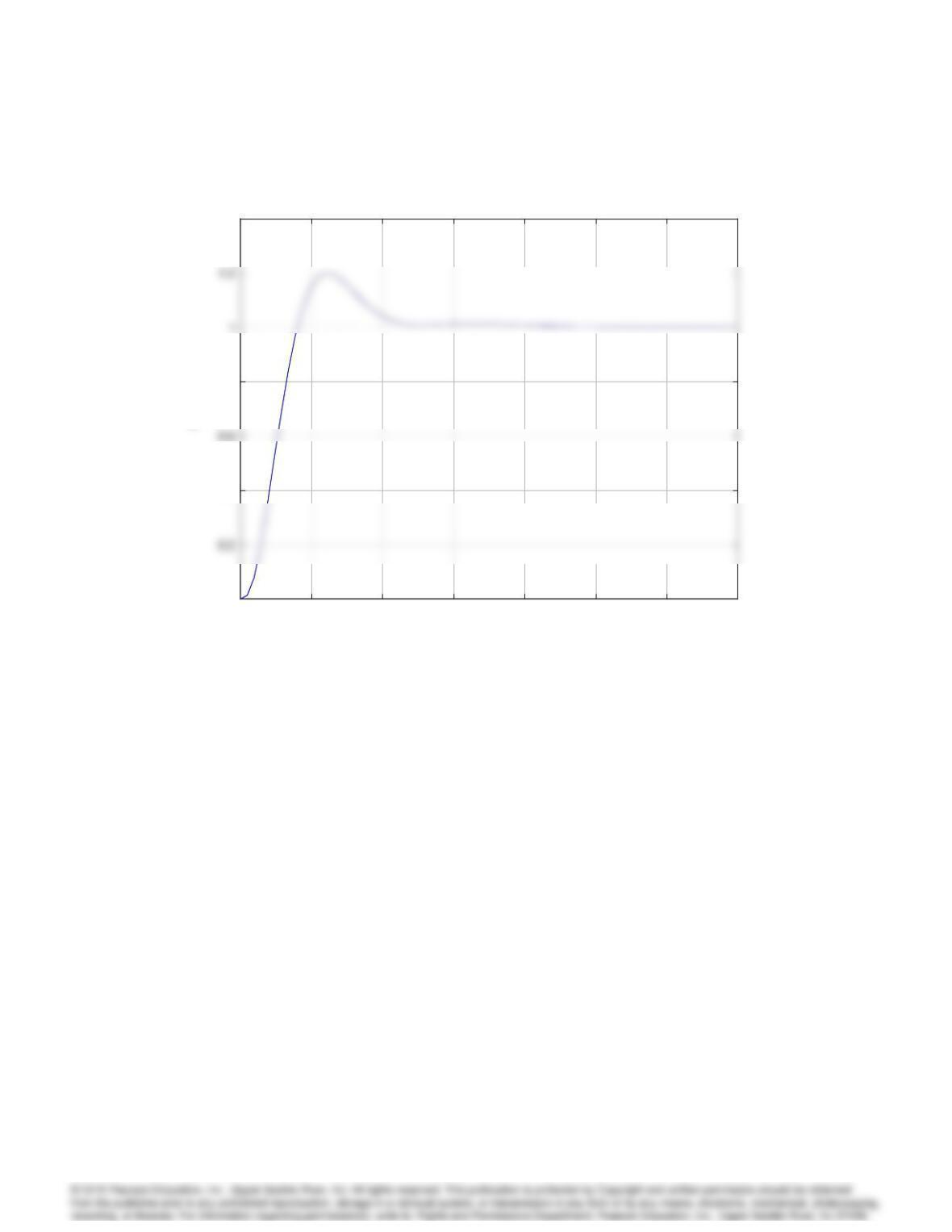
Step response of closed-loop system for Problem 10.9.
10. We have discussed three design methods: the root-locus method of Evans, the frequency-response
method of Bode, and the state-variable pole-assignment method. Explain which of these methods is
best described by the following statements (if you feel more than one method fits a given statement
equally well, say so and explain why):
1. (a) This method is the one most commonly used when the plant description must be obtained
from experimental data.
(b) This method provides the most direct control over dynamic response characteristics such
as rise time, percent overshoot, and settling time.
(c) This method lends itself most easily to an automated (computer) implementation.
(d) This method provides the most direct control over the steady-state error constants Kpand
Kv.
(e) This method is most likely to lead to the least complex controller capable of meeting the
dynamic and static accuracy specifications.
(f) This method allows the designer to guarantee that the final design will be unconditionally
stable.
(g) This method can be used without modification for plants that include transportation lag
10035
terms, for example,
G(s) = e2s
(s+ 3)2:
This method is the one most commonly used when the plant description must be obtained
from experimental data.
Solution:
(a) Frequency response method is the most convenient for experimental data because the sinu-
(b) Either the root-locus or state variable pole assignment are the most direct for control over
(c) The state variable pole-assignment is most easily programmed because, once the specifi-
(d) The frequency response method of Bode shows the error constant (either Kpor Kv) directly
(e) The root locus or Bode method will give the least complex controller. These techniques
begin with gain alone and then add network compensation only as necessary to meet
11. Lead and lag networks are typically employed in designs based on frequency response (Bode)
methods. Assuming a type 1 system, indicate the effect of these compensation networks on each
of the listed performance specifications. In each case, indicate the effect as “an increase,”
“substantially unchanged,” or “a decrease.” Use the second-order plant G(s) = K=[s(s+ 1)] to
illustrate your conclusions.
(a) Kv
(b) Phase margin
(c) Closed-loop bandwidth
(d) Percent overshoot
10036 CHAPTER 10. CONTROL-SYSTEM DESIGN: PRINCIPLES AND CASE STUDIES
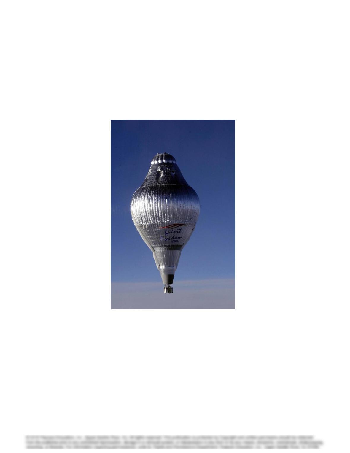
Figure 10.93: Spirit of Freedom balloon
10037
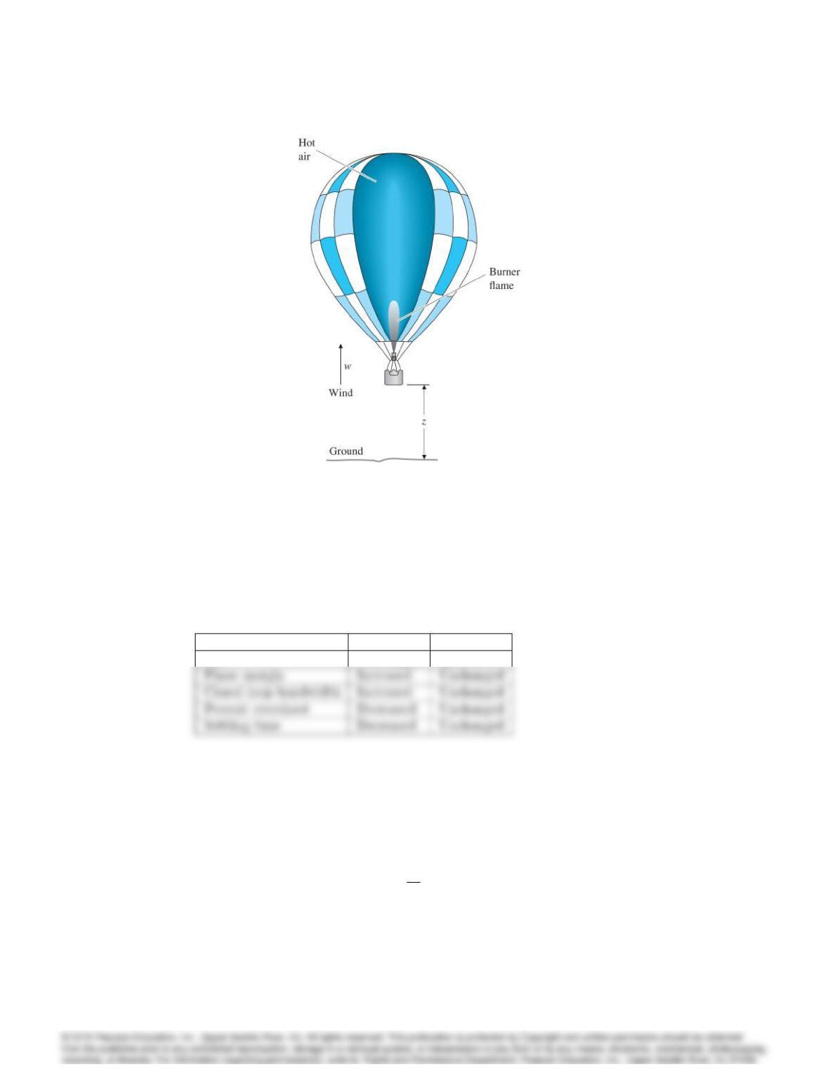
Figure 10.94: Hot-air balloon
(e) Settling time
Solution:
Lead Lag
KvUnchanged Increased
1. 12. Altitude Control of a Hot-air Balloon: American solo balloonist Steve Fossett landed in
the Australian outback aboard Spirit of Freedom on July 3rd, 2002, becoming the first solo
balloonist to circumnavigate the globe (see Fig. 10.93). The equations of vertical motion for a
hot-air balloon (Fig. 10.94), linearized about vertical equilibrium are
_
T+1
1
T =q;
2•z+ _z=aT +w;

10038 CHAPTER 10. CONTROL-SYSTEM DESIGN: PRINCIPLES AND CASE STUDIES
where
T = deviation of the hot air temperature from the equilibrium
temperature where buoyant force = weight;
z= altitude of the balloon;
q = deviation in the burner heating rate from the equilibrium rate
(normalized by the thermal capacity of the hot air);
w= vertical component of wind velocity;
1; 2; a = parameters of the equations:
An altitude-hold autopilot is to be designed for a balloon whose parameters are
1= 250 sec; 2= 25 sec; a = 0:3 m=(sec C):
Only altitude is sensed, so a control law of the form
q(s) = Dc(s)[zd(s)z(s)];
will be used, where zdis the desired (commanded) altitude.
(a) Sketch a root locus of the closed-loop eigenvalues with respect to the gain Kfor a pro-
portional feedback controller, q =K(zzd). Use Routh’s criterion (or let s=j! and
find the roots of the characteristic polynomial) to determine the value of the gain and the
associated frequency at which the system is marginally stable.
(b) Our intuition and the results of part (a) indicate that a relatively large amount of lead
compensation is required to produce a satisfactory autopilot. Because Steve Fossett was a
millionaire, he could afford a more complex controller implementation. Sketch a root locus
of the closed-loop eigenvalues with respect to the gain Kfor a double-lead compensator,
q =Dc(s)(zdz), where,
Dc(s) = Ks+ 0:03
s+ 0:122
:
(c) Select a gain Kfor the lead-compensated system to give a crossover frequency of 0.06 rad/sec.
(d) Sketch the magnitude portions of the Bode plots (straight-line asymptotes only) for the
open-loop transfer functions of the proportional feedback and lead-compensated systems.
(e) With the gain selected in part (d), what is the steady-state error in altitude for a steady
vertical wind of 1 m/sec? (Be careful: First find the closed-loop transfer function from w
to the error.)
(f) If the error in part (e) is too large, how would you modify the compensation to give higher
low-frequency gain? (Give a qualitative answer only.)
Solution:
10039
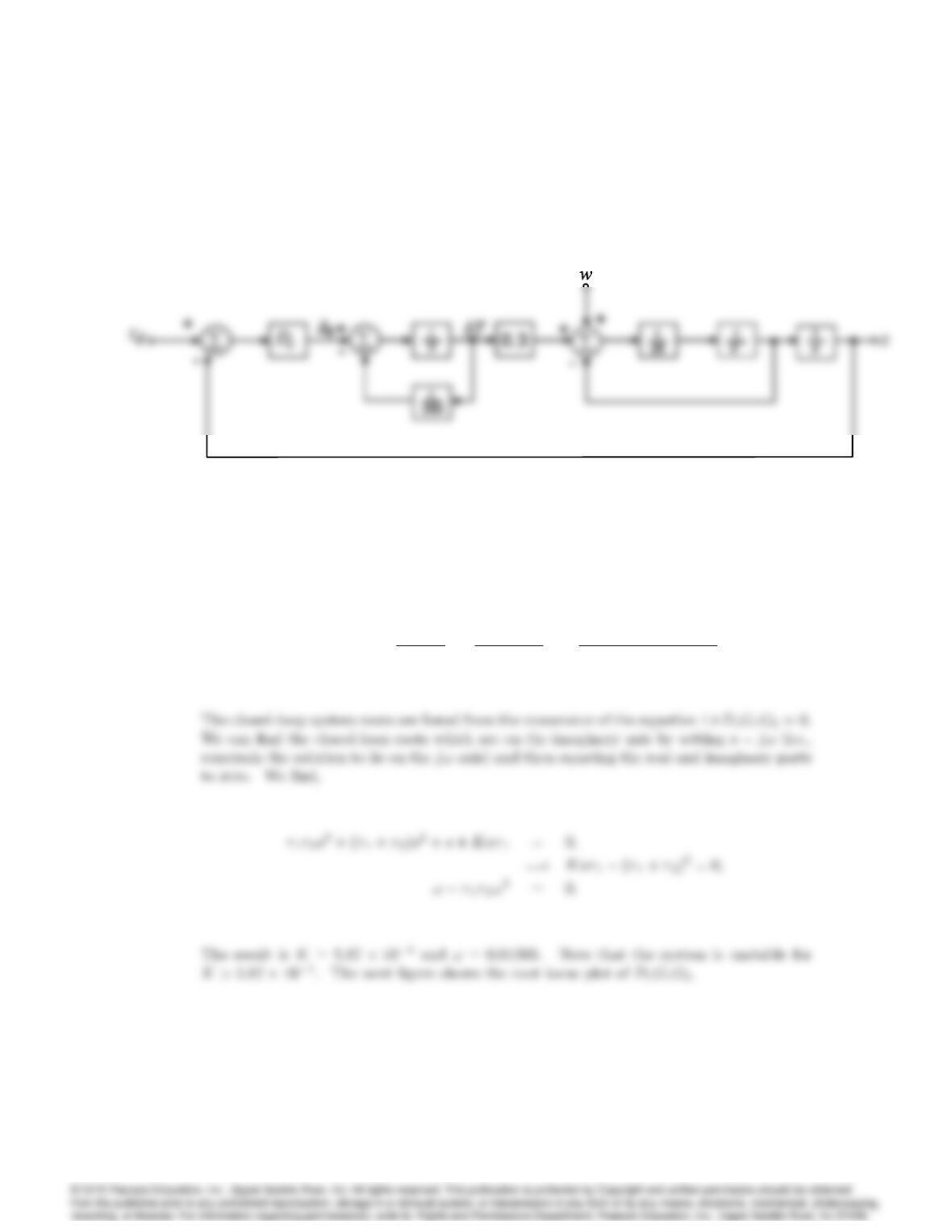
The block diagram of the system is shown below.
Problem 10.13: Block diagram for balloon problem with only altitude measurement.
1. (a) With Dc(s) = K, the open-loop transfer function is,
DcG1G2=K1
1s+ 1 a
s(2s+ 1)=75K
s(250s+ 1)(25s+ 1):