Operating Systems Chapter 10 Homework A linear model for the system was derived in the text as

10080 CHAPTER 10. CONTROL-SYSTEM DESIGN: PRINCIPLES AND CASE STUDIES

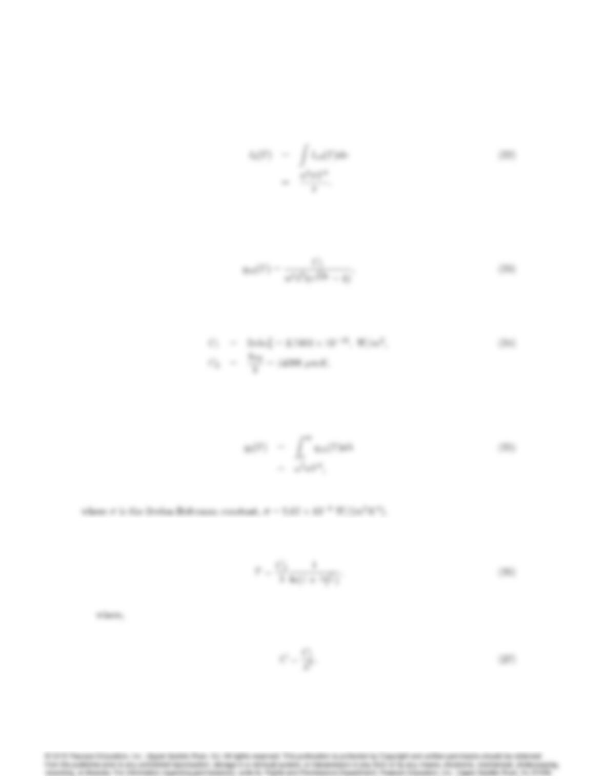
The total black-body radiation intensity, Ib, is obtained by integrating over all frequencies or

wavelength [2]

The black body emissive ‡ux is given by,

where,

Integrating over all wavelengths , we obtain the total black body emissive ‡ux [2],

The temperature may be determined from Eq. (19) as,

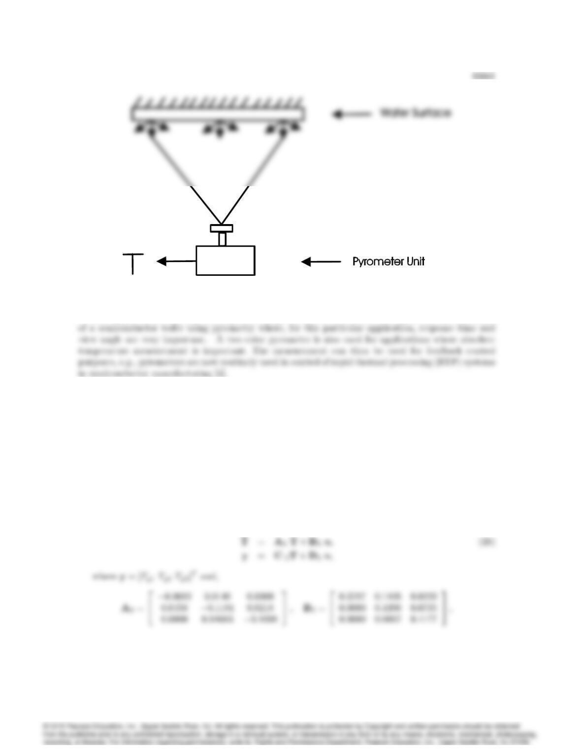
Problem 10.22: Schematic of temperature measurement using pyrometry.

The figure on the bottom of the previous page shows the schematic of temperature measurement

References:

[1] Fraden, J., Handbook of Modern sensors: Physics, Designs, and Applications, Springer, 1996.

[2] Ozisik, M. N., Radiative Transfer and Interactions with Conduction and Convection, Wiley-

Interscience, 1973.

[3] Siegel, R. and J. R. Howell, Thermal Radiation Heat Transfer, Second Ed., Hemisphere Pub-

lishing Corp., 1981.

[4] A. Emami-Naeini, et al., “Modeling and Control of Distributed Thermal Systems,” IEEE Tran.

Contrl. Syst. Tech., pp. 668-683, September 2003.

24. Repeat the RTP case study design by summing the three sensors to form a single signal to

control the average temperature. Demonstrate the performance of the linear design, and validate the

performance on the nonlinear Simulink simulation.

Solution:

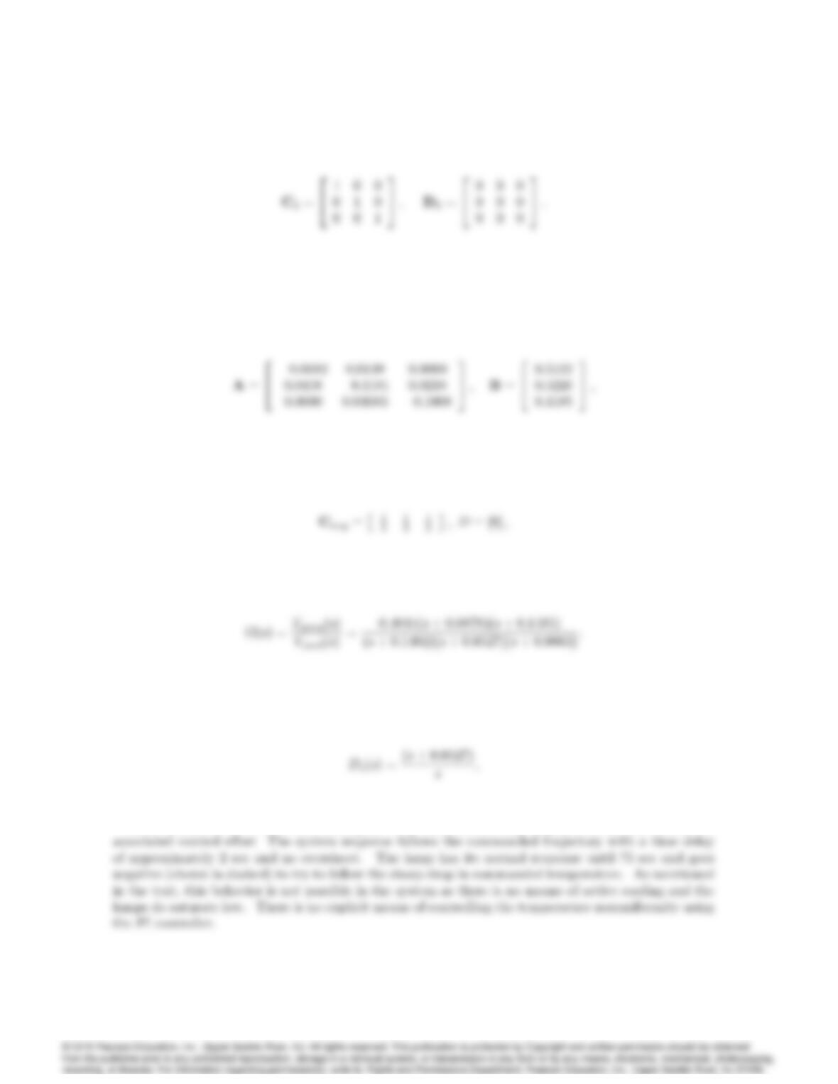
A linear model for the system was derived in the text as,

10082 CHAPTER 10. CONTROL-SYSTEM DESIGN: PRINCIPLES AND CASE STUDIES

The three open-loop poles are computed from Matlab and are located at 0:0527;0:0863;and

0:1482:Since we tied the three lamps into one actuator and are only using the average temperature

for feedback, the linear model is then:

resulting in the transfer function,

We may try a simple PI controller of the form,

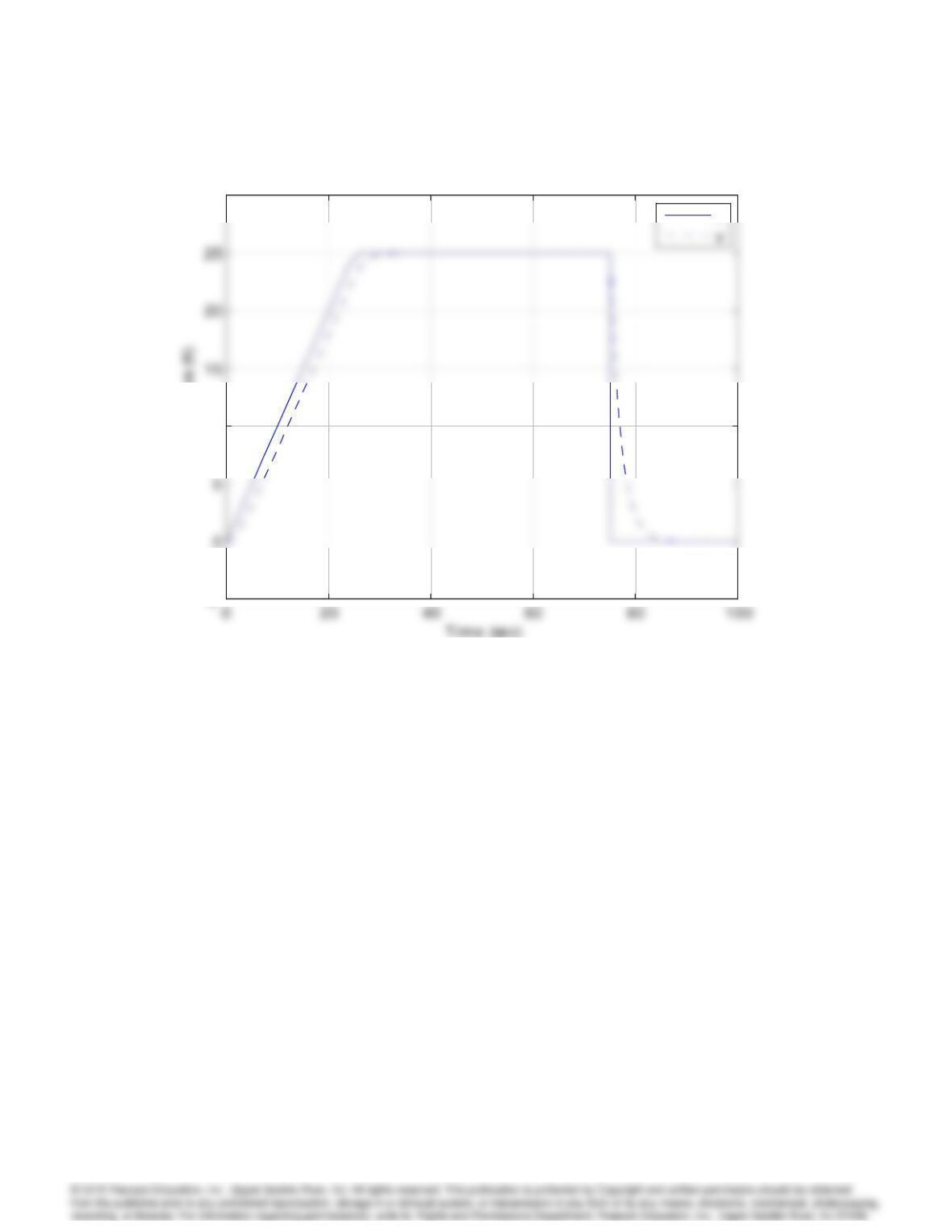
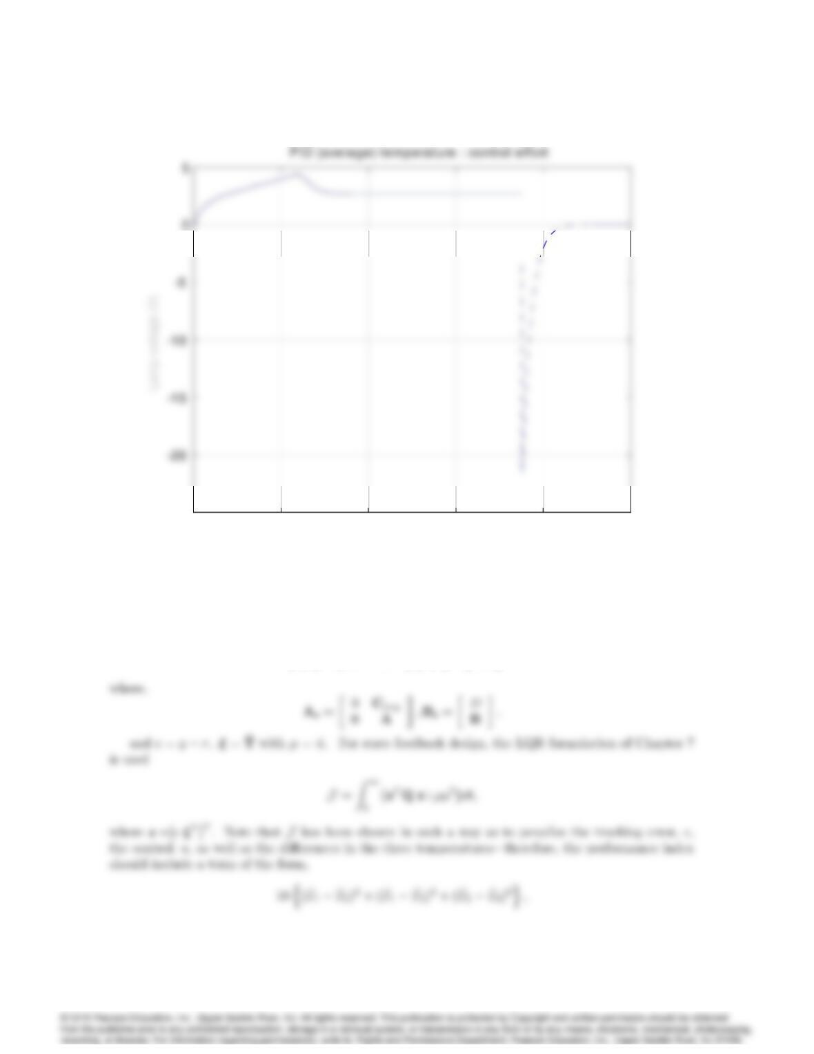
so as to cancel the effect of the slower pole. The linear closed-loop response is shown as well as the

10083

-5

10

30

Temperature (K)

PID (average) temperature tracking response

-5

10

30

Temperature (K)

PID (average) temperature tracking response

r

Problem 10.23: Linear closed-loop RTP response for PI controller.

10084 CHAPTER 10. CONTROL-SYSTEM DESIGN: PRINCIPLES AND CASE STUDIES

020 40 60 80 100

–25

Time (sec)

020 40 60 80 100

–25

Problem 10.23: RTP Linear response for PI: control effort.

Next we design a state-space based controller. As in the text, we use the error space approach for

inclusion of integral control and employ the linear quadratic gaussian technique of Chapter 7. The

error system is, _e

_

=0Cavg

0 A  e

+D

B; (29)

10085

and hence minimizes a measure of the temperature non-uniformity. As in the text, the factor of ten

is used as the relative weighting between the error state and the plant state. The state and control

weighting matrices, Qand R, are then,

The resulting feedback gain matrix computed from Matlab is,

K= [K1:K0];

where,

with xcdenoting the controller state and,

The resulting estimator gain matrix is,

3

10086 CHAPTER 10. CONTROL-SYSTEM DESIGN: PRINCIPLES AND CASE STUDIES

The closed-loop system equations are given in the text,

where ris the reference input temperature trajectory, the closed-loop state vector is xcl = [TTxT

c^

TT]Tand

the system matrices are,

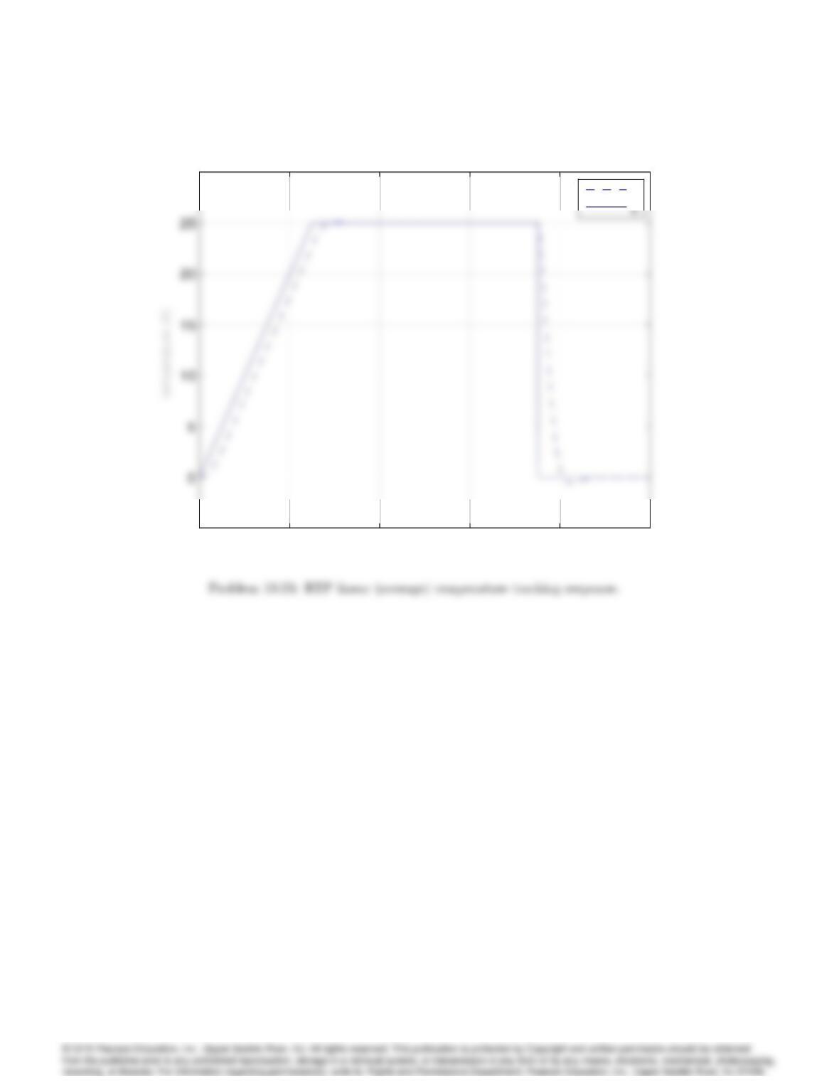
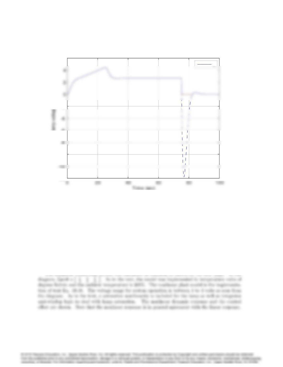
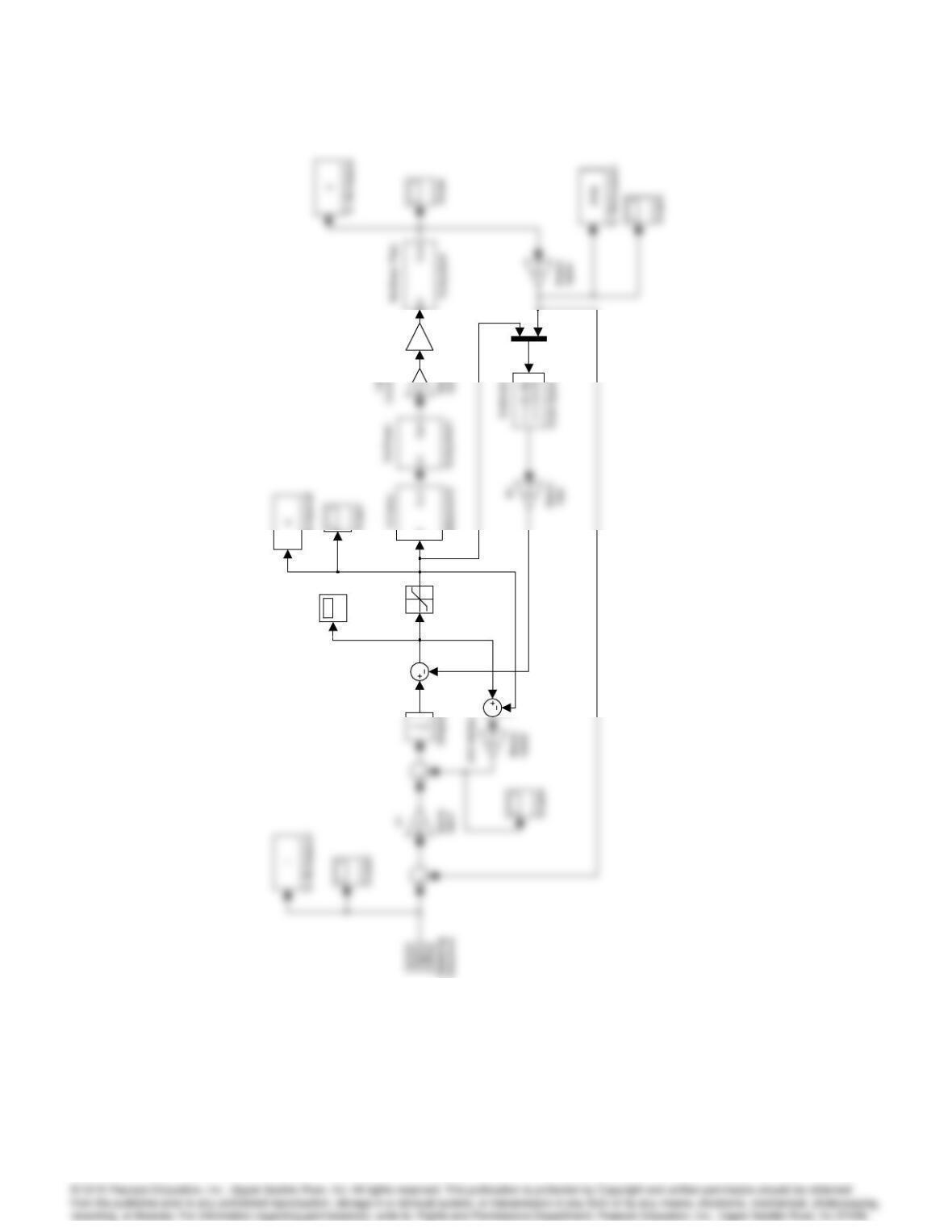
The linear closed-loop response and the associated control effort are shown. The commanded

temperature trajectory, r, is a ramp from 0C to 25C with a 1C/sec slope followed by 50 sec soak

10087

020 40 60 80 100

-5

30

Time (sec)

temperature tracking response

020 40 60 80 100

-5

30

r

10088 CHAPTER 10. CONTROL-SYSTEM DESIGN: PRINCIPLES AND CASE STUDIES

–14

–10

-6

-2

6

lamp voltage

control effort

u

–14

–10

-6

-2

6

lamp voltage

control effort

u

Problem 10.23 RTP linear (average) : control effort.

10089

To Workspace2

In1 O u t1

Subsystem2

Scope3

Scope1

Saturation

K*u

M at rix

Gain5

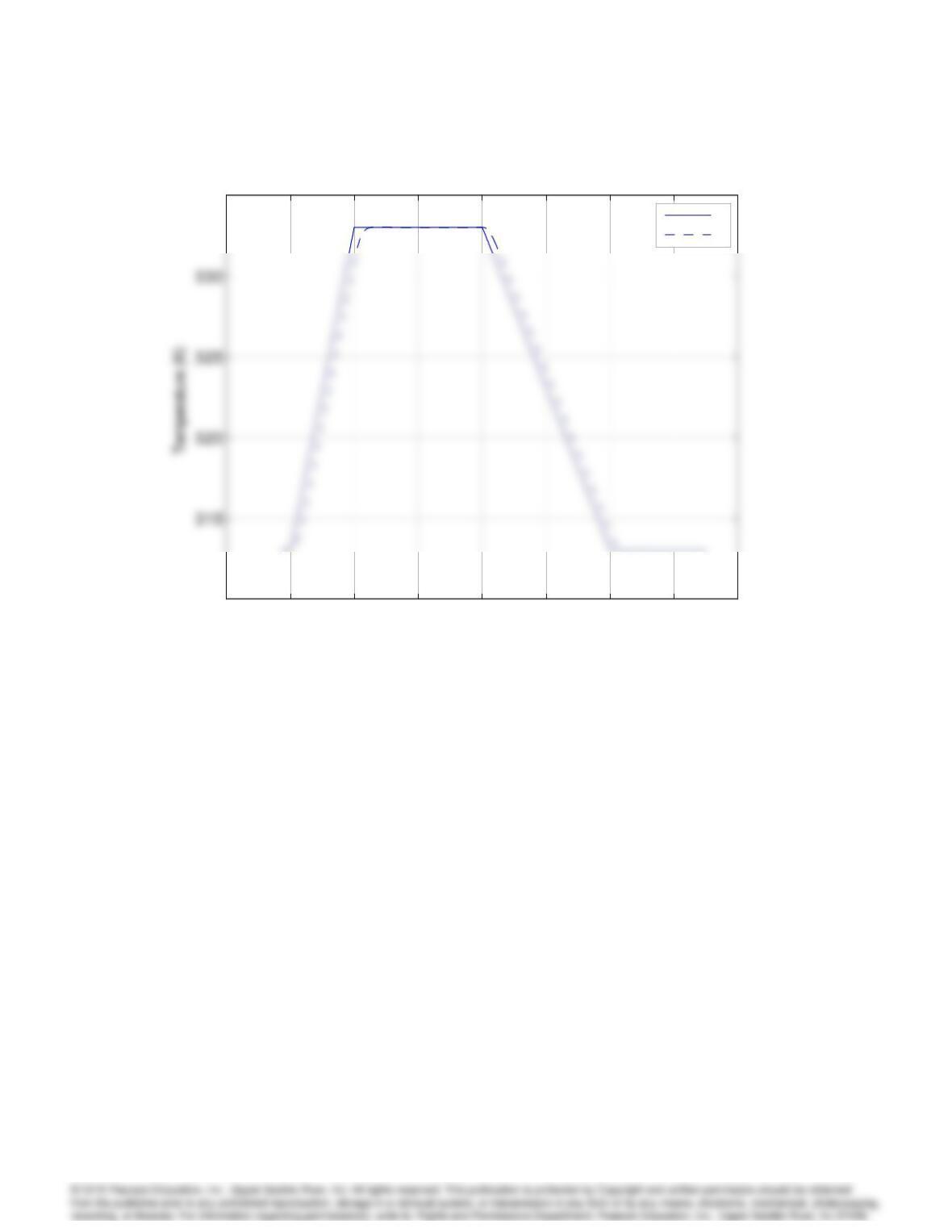
Problem 10.23: Simulink diagram for nonlinear closed-loop RTP system to control average

temperature.

10090 CHAPTER 10. CONTROL-SYSTEM DESIGN: PRINCIPLES AND CASE STUDIES

20 40 60 80 100 120 140 160 180

310

335

Time (sec)

SISO (average) temperature tracking response

r

y

20 40 60 80 100 120 140 160 180

310

335

Time (sec)

SISO (average) temperature tracking response

ry

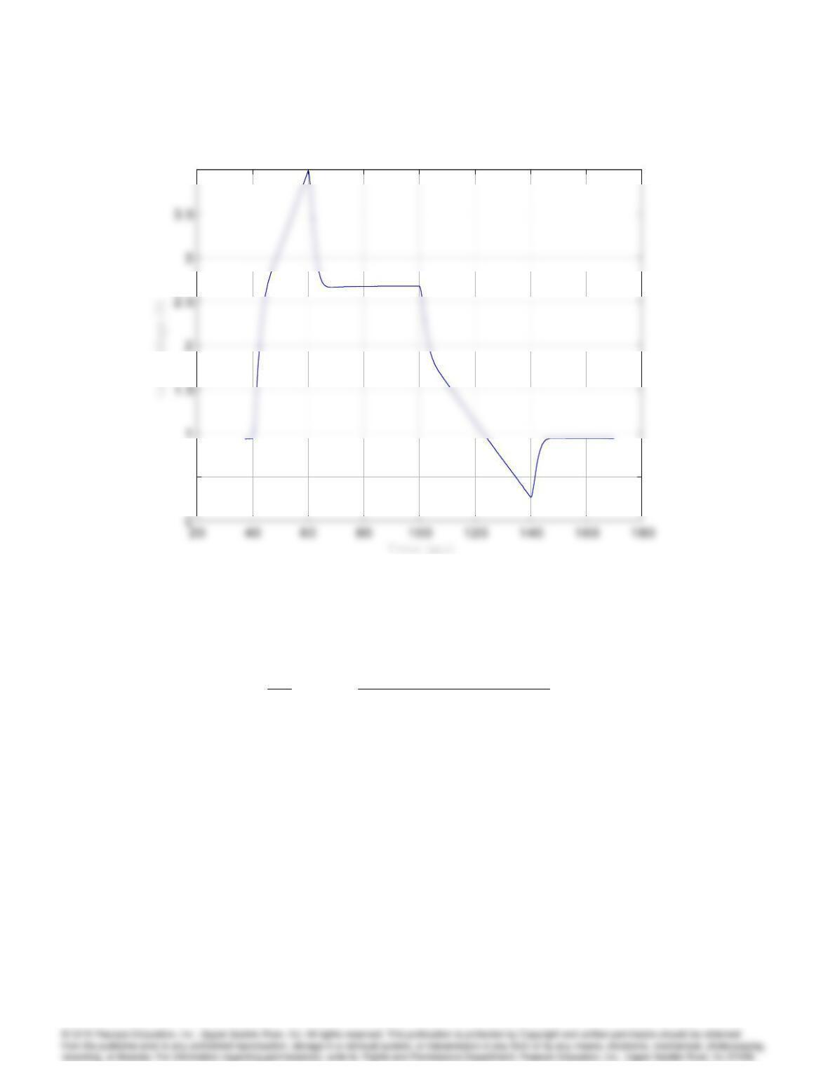
Problem 10.23: Nonlinear closed-loop response.

10091

0.5

4

SISO (average) temperature : control effort

0.5

4

Problem 10.23: Nonlinear closed-loop response: control effort.

25. One of the steps in semiconductor wafer manufacturing during photolithography is performed

by placement of the wafer on a heated plate for a certain period of time. Laboratory experiments

have shown that the transfer function from the heater power, u, to the wafer temperature, y, is given

by

y(s)

u(s)=G(s) = 0:09

(s+ 0:19)(s+ 0:78)(s+ 0:00018)

1. (a) Sketch the 180root locus for the uncompensated system.

(b) Using the root locus design techniques, design a dynamic compensator, D(s), such that

the system meets the following time-domain specifications

i. Mp5%

ii. tr20 sec

iii. ts60 sec

iv. Steady-state error to a 1C step input command <0:1C.

Draw the 180root locus for the compensated system.

Solution:

The uncompensated root locus is shown in the following figure.

10092 CHAPTER 10. CONTROL-SYSTEM DESIGN: PRINCIPLES AND CASE STUDIES

–3.5 -3 –2.5 -2 –1.5 -1 –0.5 00.5 11.5

–2.5

–1.5

-1

1.5

0.86

0.160.340.50.640.76

Root Locus

Real Axis

Uncompensated root locus.

(a) First, convert the time domain specifications to s-plane specifications:

Mp5% )&>0:707

(b) At this point there are several design methods one can use for this problem.

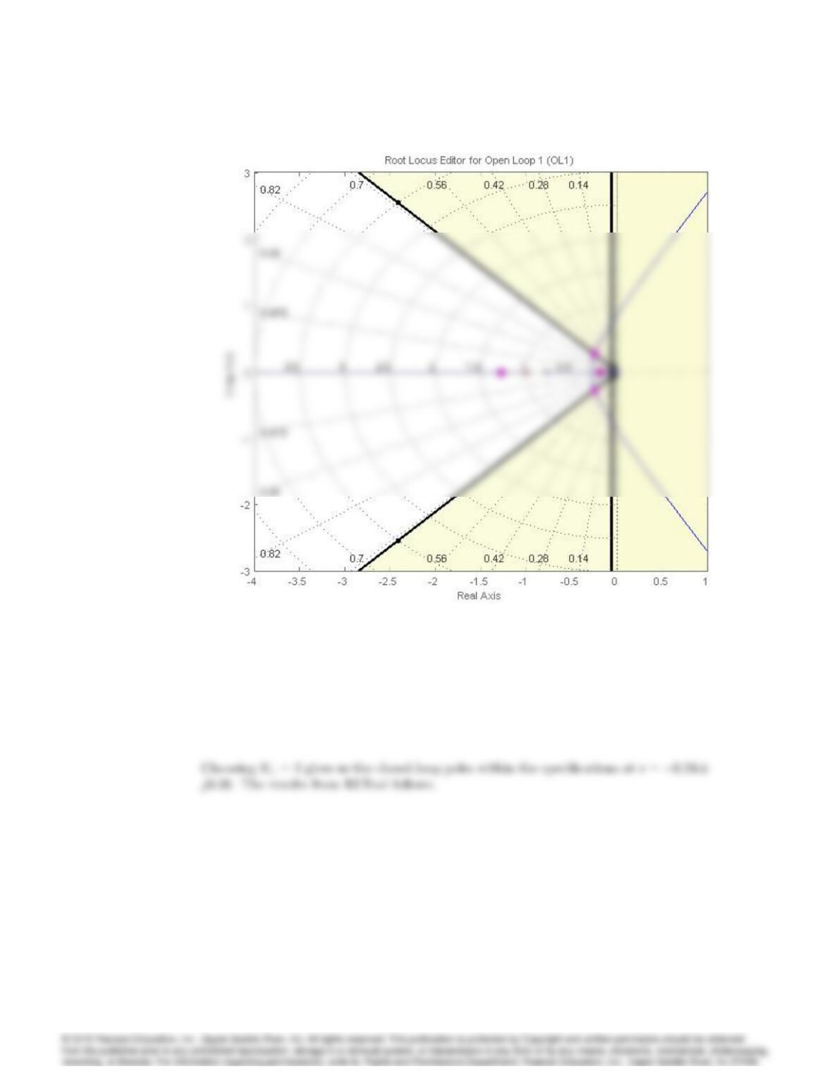
10093

RLTool: Compensator I.

10094 CHAPTER 10. CONTROL-SYSTEM DESIGN: PRINCIPLES AND CASE STUDIES

Step Response

Time (sec)

Amplitude

0 5 10 15 20 25

–0.5

2

0 5 10 15 20 25

–0.5

2

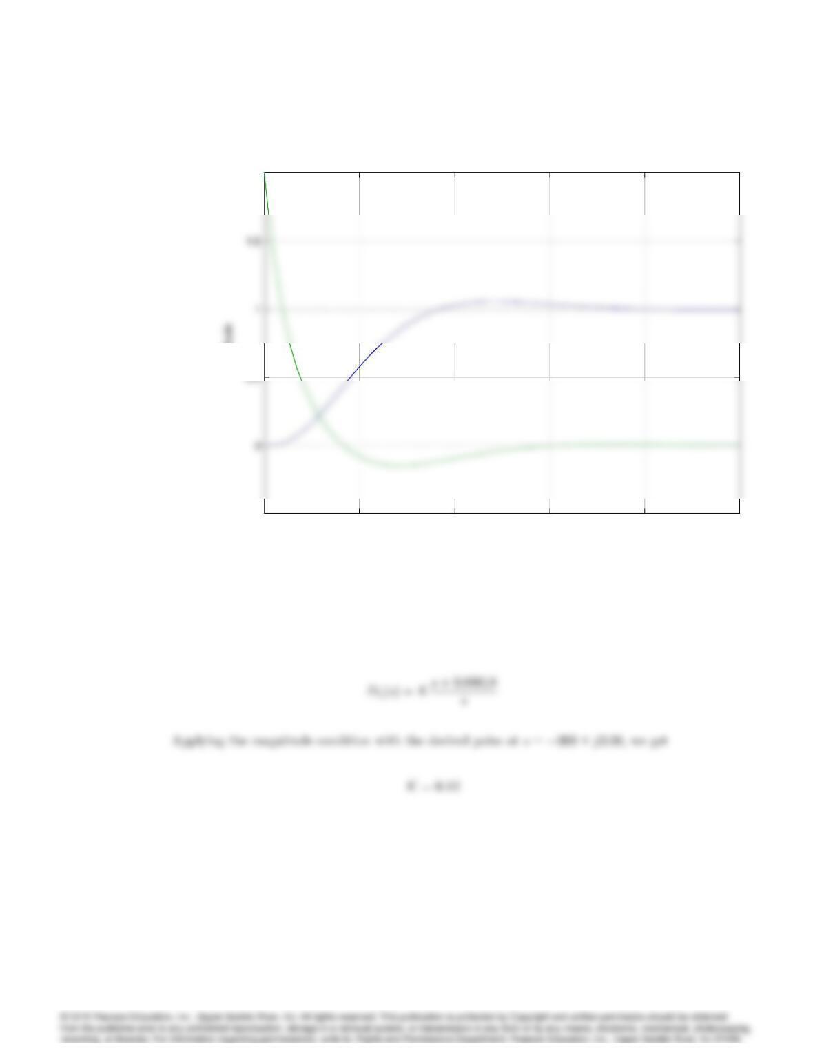
RLTool: Step response (y) and control effort (u) for Compensator I.

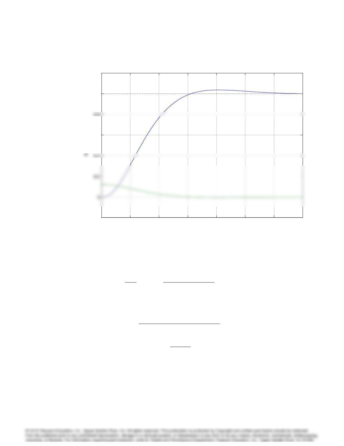
Method II: We can cancel out the nearly pure integrator with our compensator zero, and

add a pure integrator. It is possible to achieve the time domain specifications with this

compensator. The compensator becomes

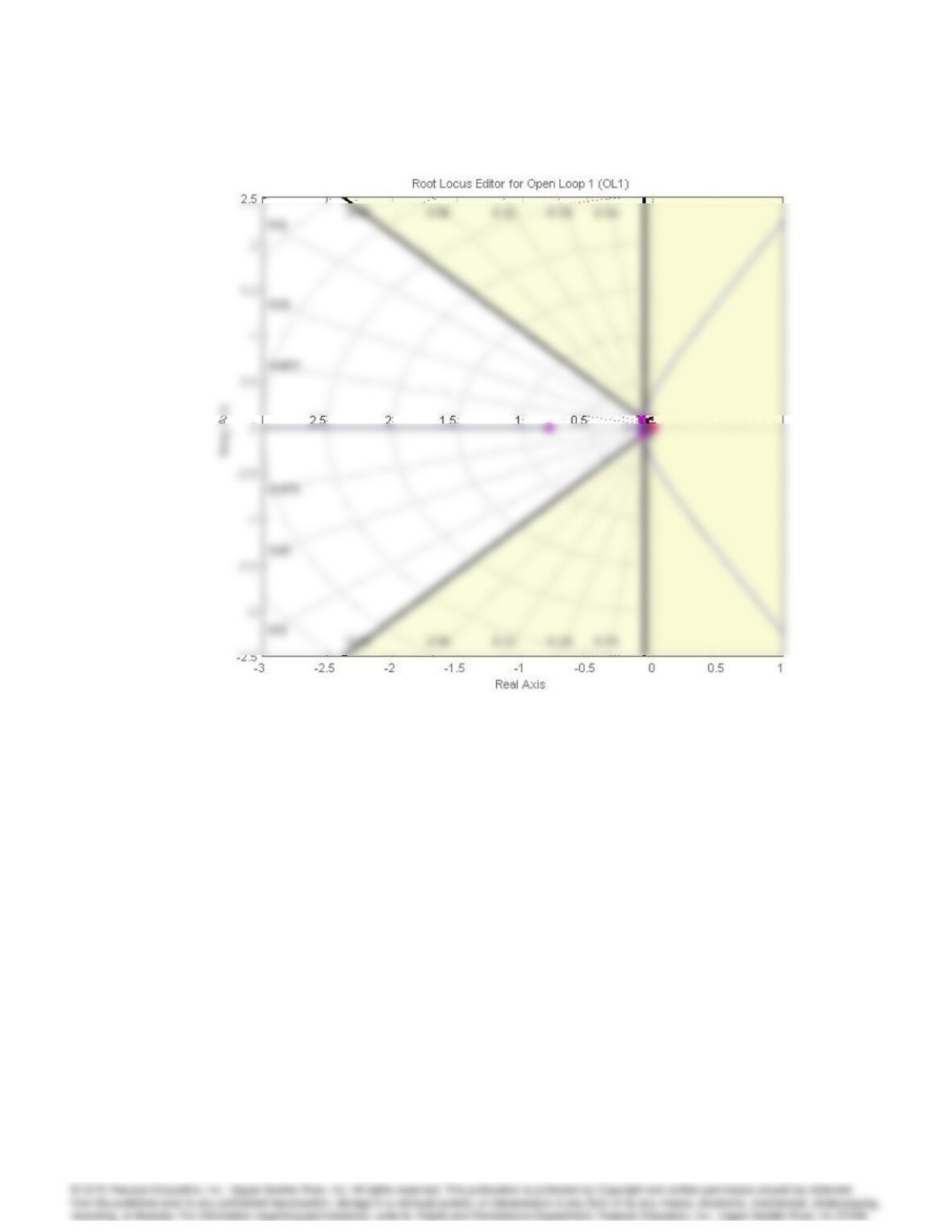
We can display the compensated root locus and s-plane regions in RLTool in the following

figure.

10095

RLTool: Compensator II.

10096 CHAPTER 10. CONTROL-SYSTEM DESIGN: PRINCIPLES AND CASE STUDIES

Step Response

Time (sec)

010 20 30 40 50 60 70

–0.2

0.6

1

1.2

010 20 30 40 50 60 70

–0.2

0.6

1

1.2

RLTool: Step response (y) and control effort (u) for Compensator II.

26. Excitation-Inhibition Model from Systems Biology (Yang and Iglesias, 2005): In Dictyostelium

cells, the activation of key signaling molecules involved in chemoattractant sensing can be modeled by

the following third order linearized model. The external disturbance to the output transfer function

is: y(s)

w(s)=S(s) = (1 )s

(s+)(s+ 1)(s+)

where, wis the external disturbance signal proportional to chemoattractant concentration, and y

is the output which is the fraction of active response regulators. Show that there is an alternate

representation of the system with the “plant” transfer function

G(s) = (1 )

s2+ (1 + +)s+ (++)

and the “feedback regulator”

Dc(s) = 

(1 )s

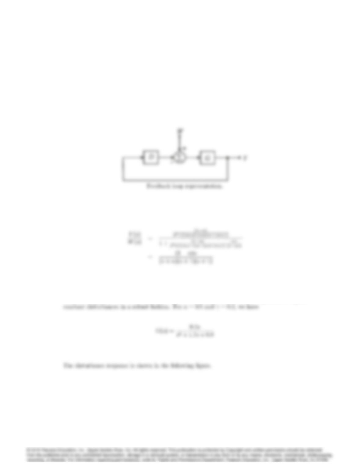
It is known that 6= 1 for this version of the model. Draw the feedback block diagram of the

system showing the locations of the disturbance input and the output. What is the significance of

this particular representation of the system? What hidden system property does it reveal? Is the

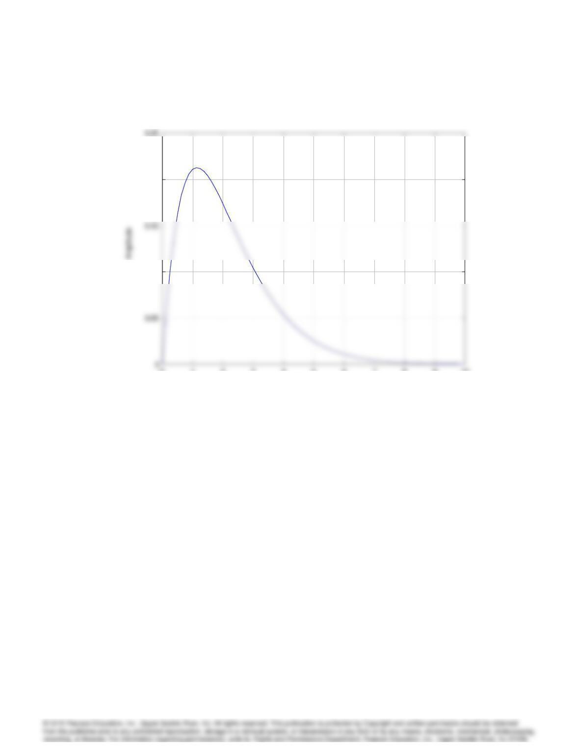
disturbance rejection a robust property for this system? Plot the disturbance rejection response of

10097

the system for a unit step disturbance input. Assume the system parameter values are = 0:5and

= 0:2.

1. Solution: From the following figure we have

The significance of this particular representation is that it reveals the internal model, namely

the pure integrator. Hence the system is Type I with respect to disturbance rejection. It rejects

10098 CHAPTER 10. CONTROL-SYSTEM DESIGN: PRINCIPLES AND CASE STUDIES

0 1 2 3 4 5 6 7 8 9 10

0.1

0.2

Step Response

Time (sec)

0 1 2 3 4 5 6 7 8 9 10

0.1

0.2

Disturbance rejection response for a unit step disturbance.