Chapter 10. Phase Diagrams
10.14. Use a mathematics application software package to
compute and plot a simple ideal solution phase diagram. Write
the program so that:
a. Input is T1
o, T2
o,• •S1
o and • •S2
o
b. Output is a plot of the two phase field.
Fix the melting points. Try several combinations of values of
• •S1
o and • •S2
o and explore the kinds of diagrams that may be
developed. Values of these parameters range around 1 (J/mole
K) for solid-solid transformations, 8 for melting and 90 for
vaporization.
Answer to 10.14.
The following program is written for MathCad.
“Compute the phase boundary compositions:”
the y axis.”
This program will compute and plot any ideal solution two phase
Chapter 10. Phase Diagrams
10.15. Use the computer program developed in Problem 10.14 as
a basis to compute and plot a phase diagram for a system
involving three phases, • •,• • and L. Identify the stable and
metastable portions of this diagram.
Answer to 10.15.
So that
Chapter 10. Phase Diagrams
——–————————–———-——————-——-
10.16. The system A-B obeys the simple regular solution model.
A melts at 1352 K with an entropy of fusion of 6.9 (J/mole K);
B melts at 1148 K with an entropy of fusion of 8.5. (J/mole K).
phase a0
• •
= -11,400 (J/mole). Find the compositions of the
boundaries of the two phase (• • + L) field at 1300 K. (Note: this
will require solution of two simultaneous nonlinear equations;
standard mathematics applications packages have this feature.)
Answer to 10.16.
“Compute the free energies of the transformations at T:
“Start with “Guess values” for the variables sought; MathCad
uses them as a starting point in the iterative process it uses to find
a solution.“
Given
Chapter 10. Phase Diagrams
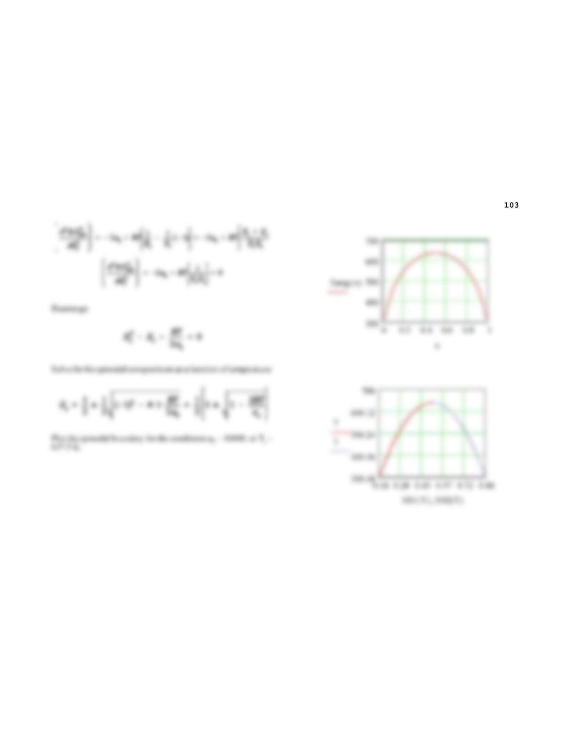
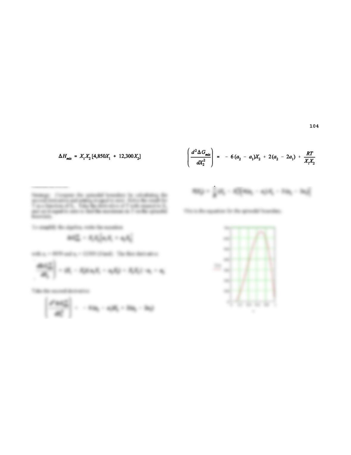
10.17. Compute and plot the phase boundaries and the spinodal
boundaries for a solution that obeys the model
Answer to 10.17.
Program and plot this result, see below.
Find the second derivative and set it equal to zero:
Chapter 10. Phase Diagrams
———–—————-——–——-————————–
Chapter 10. Phase Diagrams
10.18. Find the critical temperature for the miscibility gap that
will be found in a regular solution with
Answer to 10.18.
Add to this the second derivative of the ideal mixing term:
Set the second derivative equal to zero and solve for T:
Chapter 10. Phase Diagrams
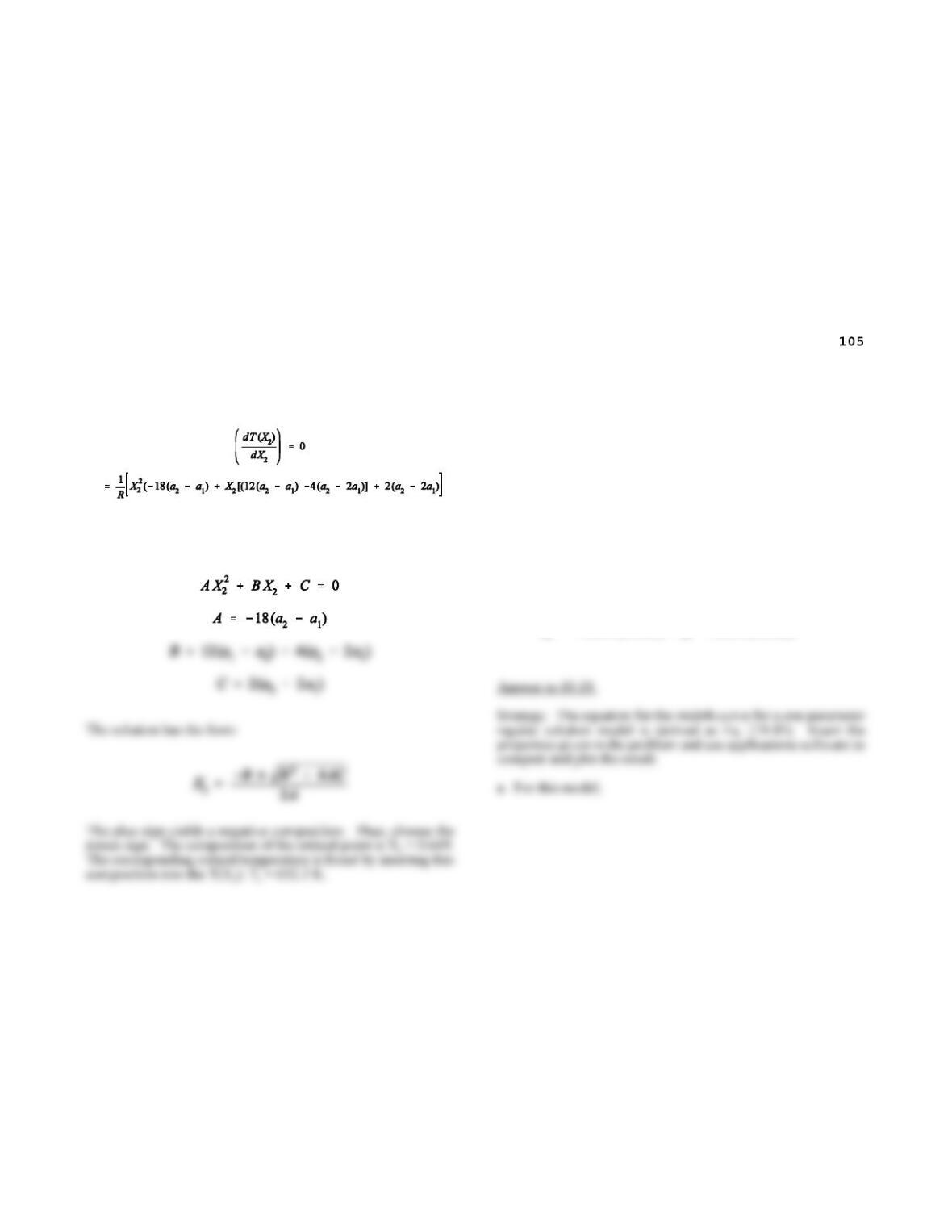
To find the critical temperature, take the derivative of T(X2) and
set it equal to zero:
To find the coordinates of the maximum solve this quadratic
equation for X2. This is an equation of the form:
———–—————-——–——-—————————
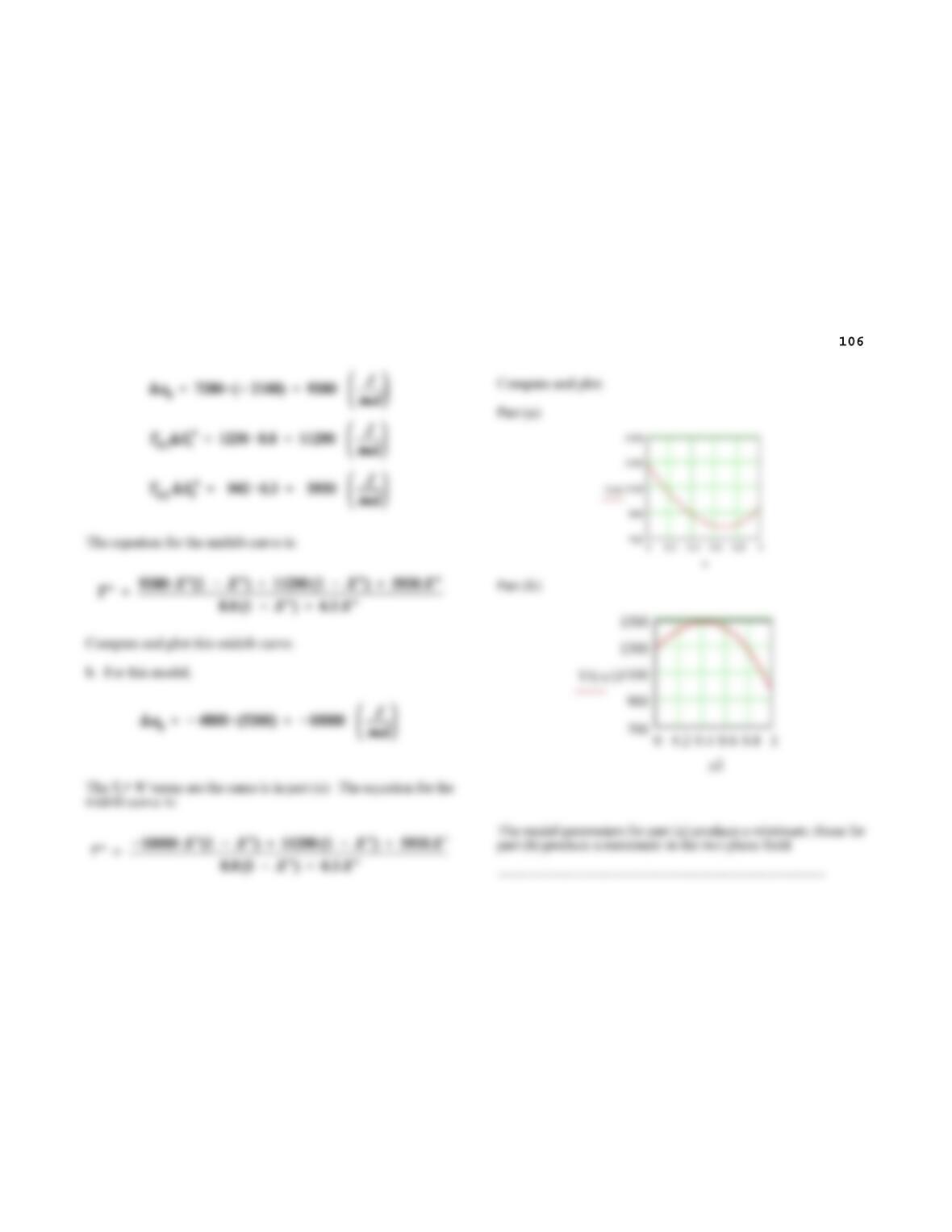
10.19. Compute and plot the midrib curves for the (• • + L) fields
for two systems with the following properties:
a. T0k K • •Sk
o (J/mole K)
Component 1 1283 8.8
Component 2 942 6.3
a0
• •
= 7,280 (J/mole) a0
L = – 2,100 (J/mole)
b. T0k K • •Sk
o (J/mole K)
Component 1 1283 8.8
Component 2 942 6.3
a0
• •
= – 4,800 (J/mole) a0
L = 5,200 (J/mole)
Chapter 10. Phase Diagrams
Chapter 10. Phase Diagrams
10.20. At 1550 K the solubility of oxygen in zirconium is
estimated to be 120 ppm. The Zr-O system forms a very stable
compound, ZrO2, an important ceramic refractory. No other
oxides are stable at 1550 K. Estimate the Henry’s law coefficient
Answer to 10.20.
gram atom is –80,280/3 = -26,760 (J/mol). The common tangent
line passes negligibly close to the origin for the dilute terminal
phase; its equation is of the form y = mx + b with b = 0. The
intercept on the O side of the diagram occurs at
The slope of the tangent line is given by
Chapter 10. Phase Diagrams
10.21. Assuming that the liquid solution of oxygen in silicon is
an ideal solution, estimate the melting point of quartz, a crystal
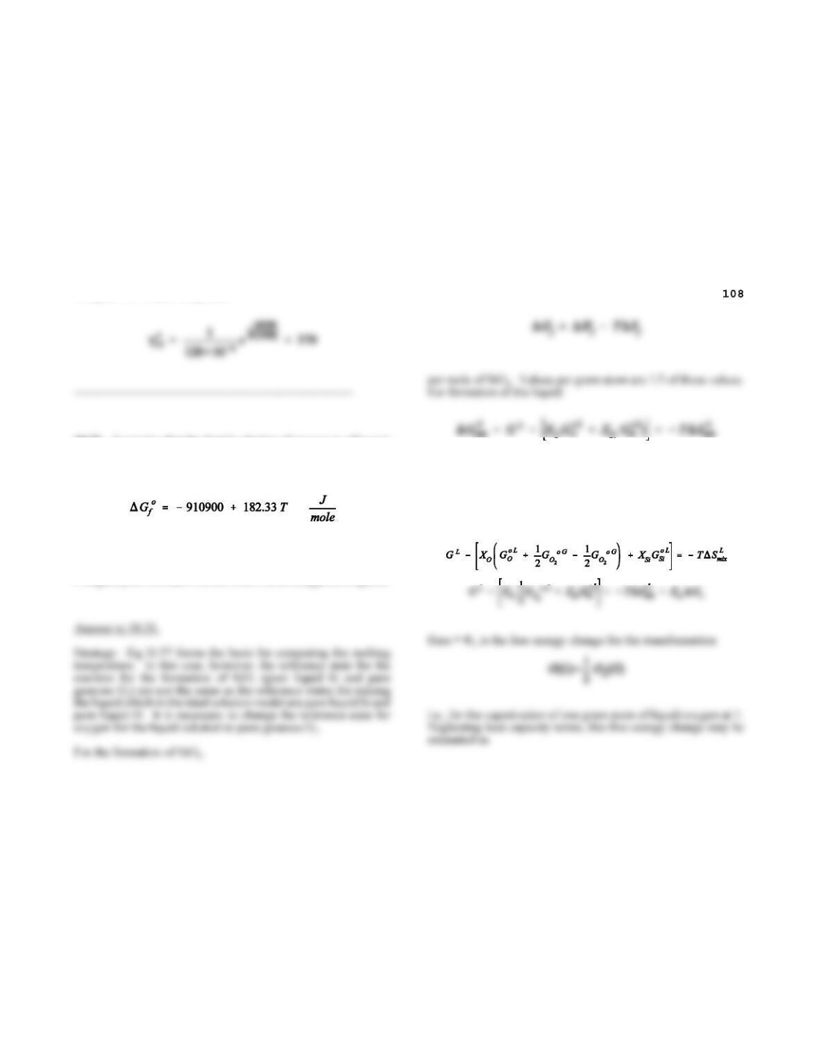
form of silica (SiO2). The free energy of formation of quartz is
Note carefully that the reference states in this relation are crystal
silicon and gaseous oxygen. Estimate the melting point of quartz.
Compare your estimate with the observed melting point of quartz.
where • •Smix
L is the ideal entropy of mixing. Change the
reference state for oxygen in this equation from O in the liquid to
O2 as a gas. Add and subtract the free energy of the new
reference state:
Chapter 10. Phase Diagrams
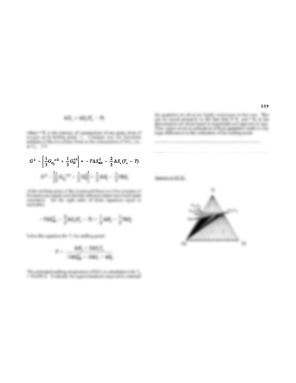
10.22. Consider the potential – composition diagram for the Fe-
Cr-O system shown in Figure 10.33. Replot this diagram on the
Gibbs triangle. Plot the tie lines in the two phase fields
quantitatively.