4I
L
2
6I
L
A
L
3
12 I
L
= 2.344 10–6,
4I
L
= 5 10–5
2
6I
L
= 9.375 10–6,
A
L
= 1.25 10–3
56
6
2
1.875 10 0 9.375 10
210 10 1.0 10 0
{}f
Actual forces
{}f
=
0
[ ] { } – { }k d f
1x
f
= 23.8 – 0 = 23.8 kN
1y
f
= – 2.74 + 20.0 = 17.26 kN
Element (3)
0
2x
f
= 17.55 kN
f
227
Calculate [k]’s based on node 2 and 3 contributions as
Element (1)
C = 0, S = 1
2
12 6
(3)
0
0
4
Symmetry
II
L
L
LI
Element (2)
C = 1, S = 0
E
22
12 16 12 6
6
(2) (3)
0 0 0 0
0
I I I I
LL
LL
I
AA
229
2
12 I
L
=
4
2
12(2 10 )
4
= 1.5 10–4 m2
6I
L
=
4
6(2 10 )
4
= 3.0 10–4 m3
E
L
=
6
210 10
4
= 5.25 107
kN
m
[k(1)] = 5.25 107
2 2 2
44
2
4
1.5 10 0 3 10
2 10 0
8 10
uv
2
12 I
L
=
4
2
12(2 10 )
5
= 9.6 10–5 m2
6I
L
=
4
6(2 10 )
5
= 2.4 10–4 m3
m
E
6
210 10
kN
4
Symmetry 8 10
Assemble global equations for node 2
0
0
600
= 107
23
2
13
2
32
8.48 10 0 1.58 10
1.05 10 1.01 10
Symmetry 7.56 10
u
v
Solving simultaneously
u2 = – 1.486 10–4 m, v2 = – 7.674 10–5 m
2 = 7.978 10–3 rad
Element forces
{}f
=
[]k
[T] {d}
[T] {d} =
4
5
3
0
0 1 0 0 0 0
0
1 0 0 0 0 0
0
0 0 1 0 0 0
1.486 10
0 0 0 0 1 0
0 0 0 1 0 0 7.674 10
0 0 0 0 0 1 7.978 10
{}f
=
(1)
[]k
5
4
3
0
0
0
7.674 10
1.486 10
7.978 10
{}f
= 5.25 107
2
44
44
5
2
4
44
3
44
: : : 2 10 0 0 0
0
. . . 0 1.5 10 3 10
0
. . . 0 3 10 4 10
7.674 10
. . . 2 10 0 0
1.486 10
. . . 0 1.5 10 3 10
7.978 10
: : : 0 3 10 8 10
Multiplying matrices yields
(1)
11xx
(1)
22
xx
(1)
1y
(1)
2y
(1)
1
m
= 165.2 kN m,
(1)
2
m
= 335.1 kN m
Similarly for element (2)
(2)
(2) (2) (2)
2x
3x
(2)
2y
f
= 80.58 kN =
(2)
3y
f
(2)
2
m
= 264.8 kN m,
(2)
3
m
= 138.0 kN m
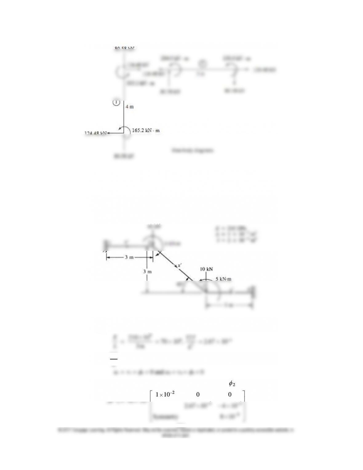
231
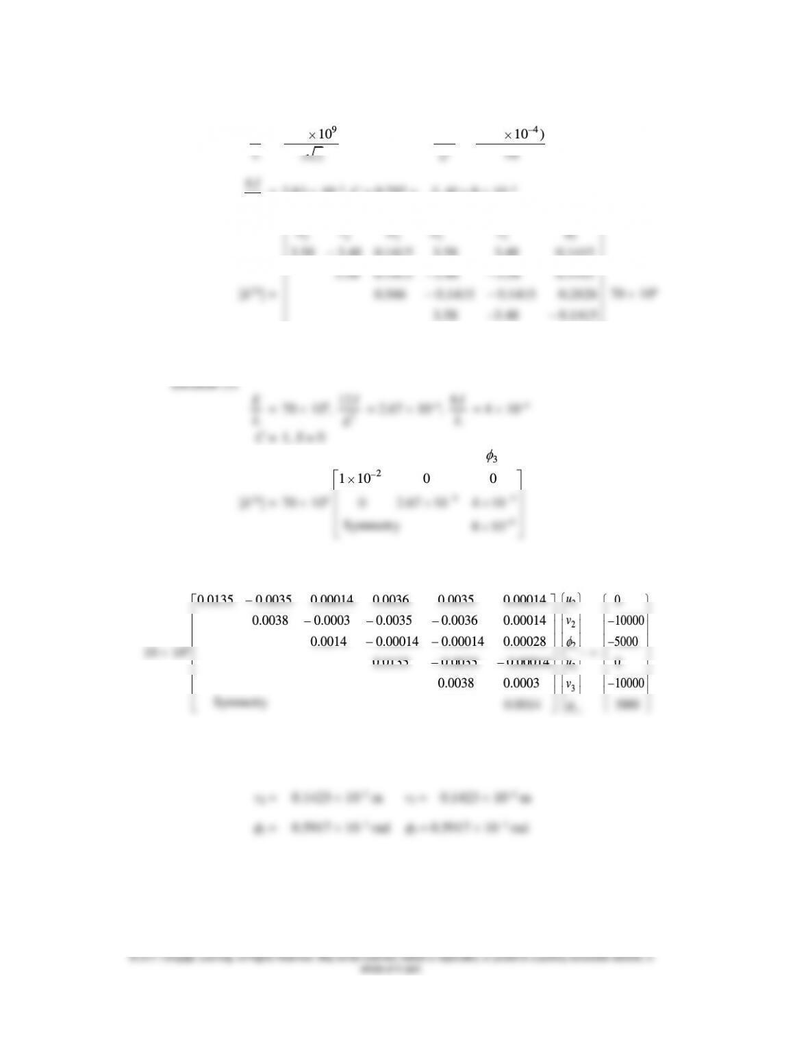
5.10
Element (1)
E
L
9
210 10
3m
2
12 I
L
6I
L
= 4 10–4, C = 1, S = 0
44
–4
2.67 10 4 10
Symmetry 8 10
Element (2)
E
L
=
9
210 10
32
= 49.5 109,
2
12 I
L
=
4
12(2 10 )
18
= 1.33 10–4
6I
L
= 2.83 10–4, C = 0.707 = – S, 4I = 8 10–4
E
L
2
12 I
3 3 3
2 2 2
3.58 3.48 0.1415 3.58 3.48 0.1415
3.58 0.1415 3.48 3.58 0.1415
uv
u v d
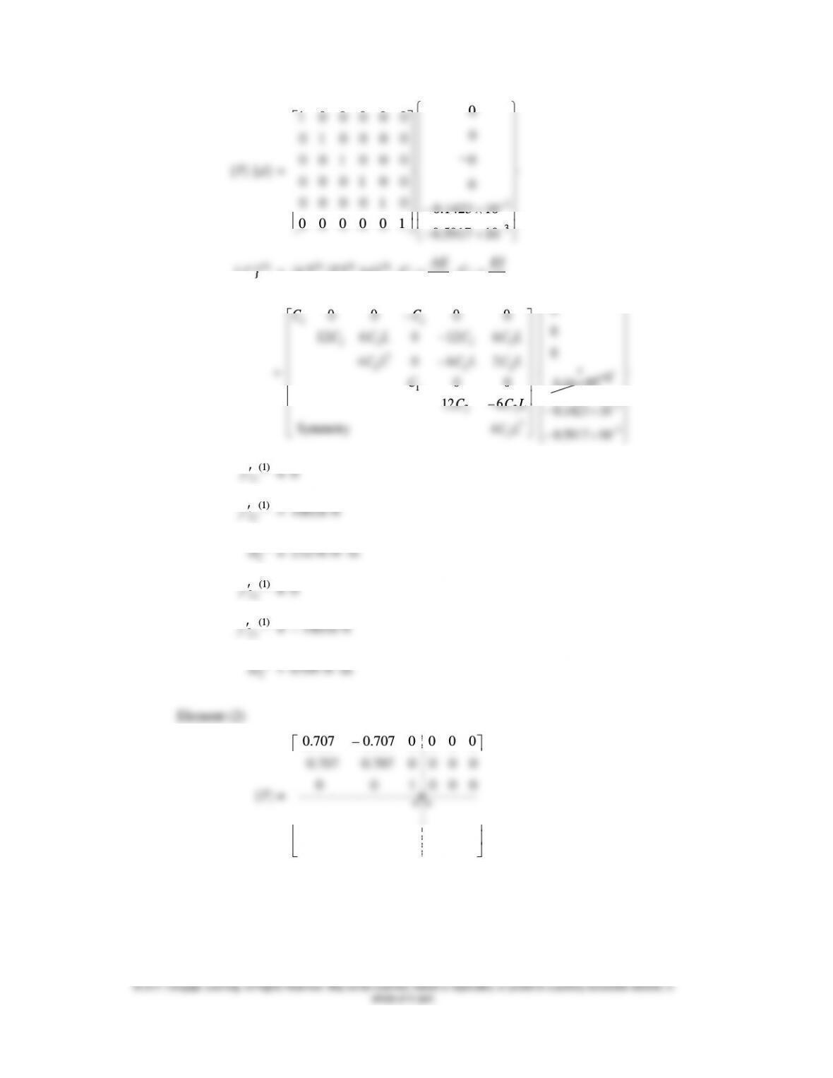
2
3
0
100000
0
0 1 0 0 0 0
~
0 0 1 0 0 0 0
0 0 0 1 0 0 0
0 0 0 0 1 0 0.1423 10
000001 0.5917 10
(1)
{}f
=
(1) (1) (1)
12
3
[ ] [ ] { } , ,
AE EI
k T d C C
LL
11
2 2 2 2
2
2 2 2
0 0 0 0
12 6 0 12 6
4 0 6 2
CC
C C L C C L
C L C L C L
0
0
0
234
(2)
{}f
=
(2) (2) (2)
[ ] [ ] { }k T d
=
4
4
0
0.387 10 0
11,720
0
0.387 10 0
11,720
where
(2)
[]k
from Equation (6.1.8) text
10
2
3
11
2
3
0.16 10 0
0.1423 10
0.5917 10
0.85 10 0
0.1423 10
0.5917 10
Similarly for element (3)
f
(3)
3x
(3)
3y
f
= – 10,028 N
(3)
3
m
= – 6709 N m
(3)
4x
f
= 0
(3)
4y
f
= 10,028 N
(3)
4
m
= – 23276 N m
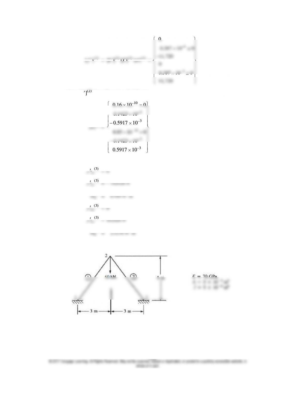
5.11
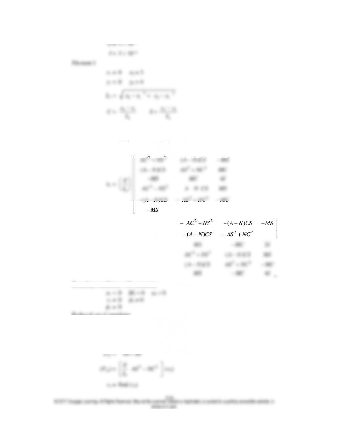
Figure P5–11
This problem is done using symmetry and Mathcad
E = 70 109
A = 3 10–2
I = 3 10–4
Element 1
x1 = 0 x2 = 3
y1 = 0 y2 = 4
L1 =
22
2 1 2 1
x x y y
C =
21
1
xx
L
S =
21
1
yy
L
C = 0.6 S = 0.8
N =
2
1
12I
L
M =
1
6I
L
E
22
22
()
()
4
AC NS A N CS MS
A N CS AS NC MC
MS MC I
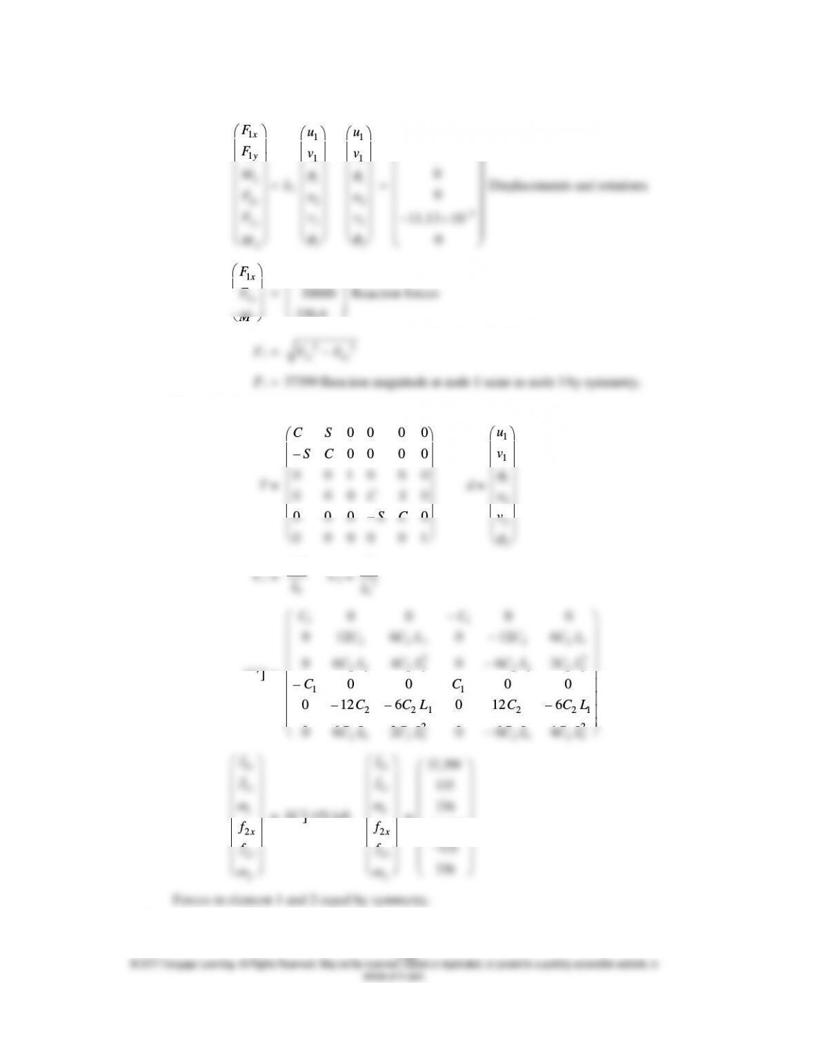
v2 = – 11.13 10–5 m Displacement of node 2
1
1
1
2
2
2
x
y
x
y
F
F
M
F
F
M
1
1
1
2
2
2
u
v
u
v
1
1
1
2
2
2
u
v
u
v
5
0
0
0
0
11.13 10
0
1
x
F
22331.7
Forces in elements
0 0 0 0
0 0 0 0
0 0 1 0 0 0
0 0 0 0
0 0 0 0
0 0 0 0 0 1
CS
SC
CS
SC
1
1
1
2
2
2
u
v
u
v
C1 =
1
AE
L
C2 =
3
1
EI
L
[]k
=
11
2 2 1 2 2 1
22
2 1 2 1 2 1 2 1
11
2 2 1 2 2 1
22
2 1 2 1 2 1 2 1
0 0 0 0
0 12 6 0 12 6
0 6 4 0 6 2
0 0 0 0
0 12 6 0 12 6
0 6 2 0 6 4
CC
C C L C C L
C L C L C L C L
CC
C C L C C L
C L C L C L C L
1
1
1
2
2
2
x
y
x
y
f
f
m
f
f
m
=
[]k
[T] {d}
1
1
1
2
2
2
x
y
x
y
f
f
m
f
f
m
=
37,399
135
336
37,399
135
336
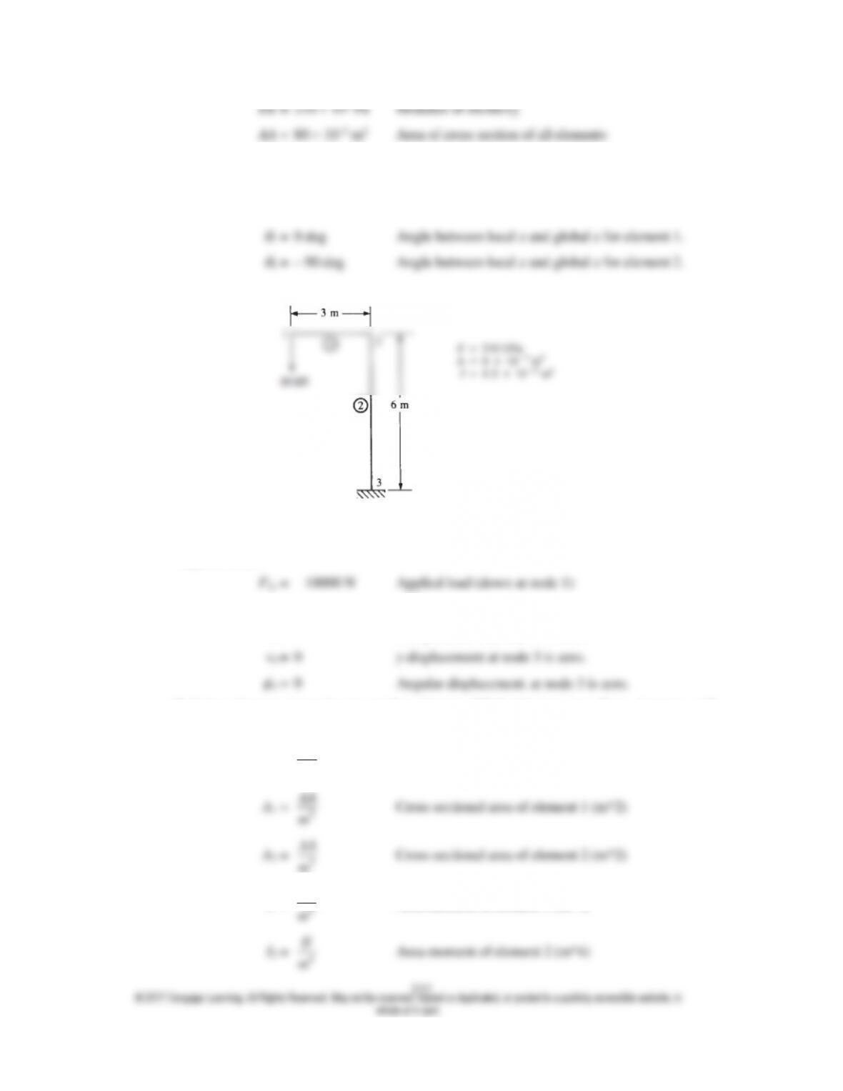
5.12 Determine displacements and rotations of the nodes, element forces, and reactions.
EE = 210 109 Pa Modulus of elasticity
AA = 80 10–3 m2 Area of cross section of all elements
II = 1.2 10–4 m4 Area moment of inertia of all elements
LL1 = 3 m Length of element 1
LL2 = 6 m Length of element 2
Figure P5.12
Applied loads
Boundary conditions
u3= 0 x-displacement at node 3 is zero.
Defining element properties in unitless format. (Mathcad does not allow elements with
dissimilar units within the same matrix.)
E =
EE
Pa
Modulus of elasticity (Pa).
AA
2
m
I1 =
4
II
m
Area moment of element 1 (m^4)
4
II
m
L1 =
1
LL
m
Length of element 1(m)
L2 =
2
LL
m
Length of element 2 (m)
C1 = cos (
1) Cosine of angle between local x and global x for
element 1.
S1 = sin (
1) Sine of angle between local x and global x for element
1.
2.
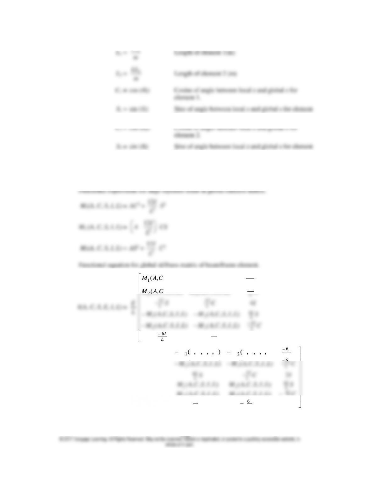
Functional equations for the global stiffness matrix for a 2D beam/frame element with axial
effects.
Refer to text Equation (5.1.11)
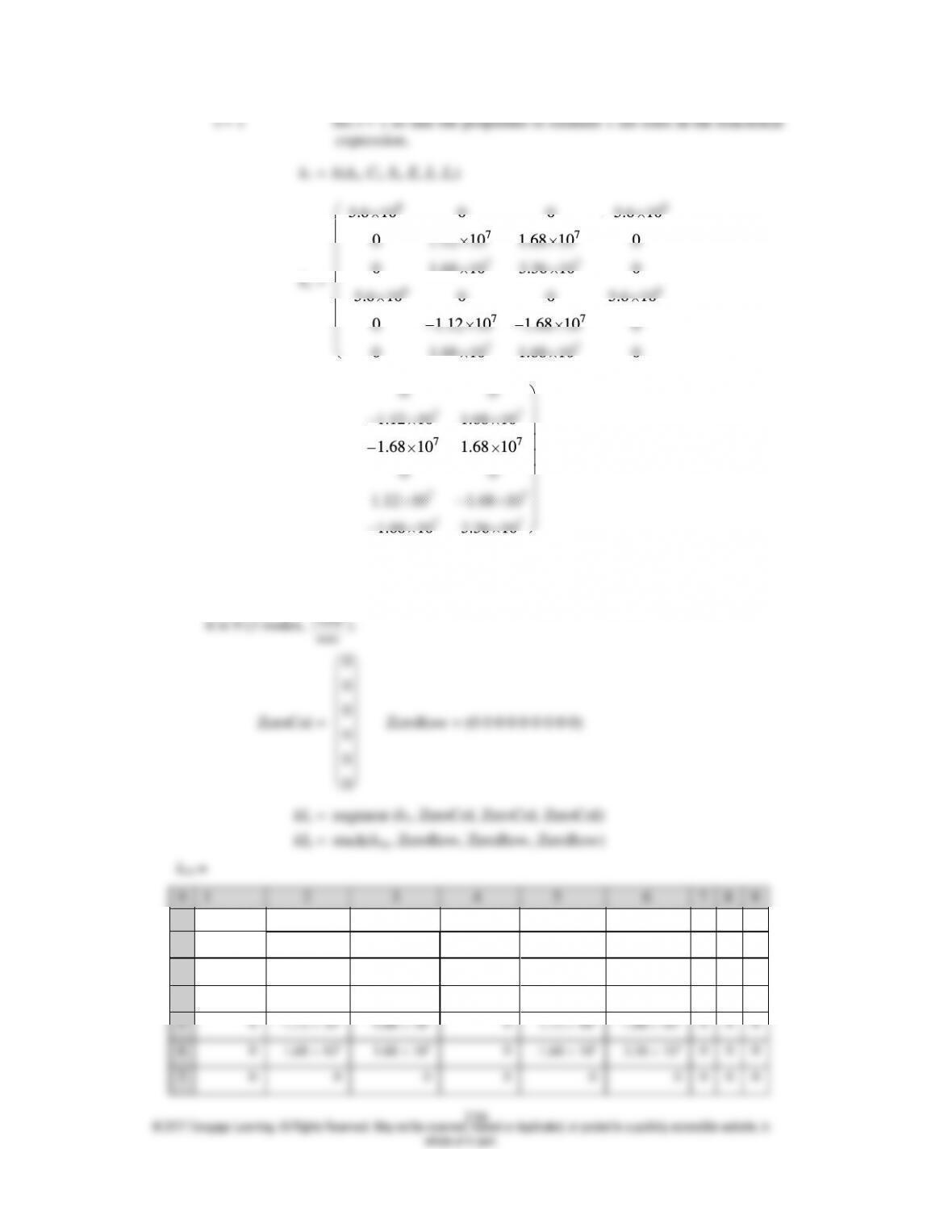
i = 1 Set i = 1 so that the properties of element 1 are used in the functional
expression.
k1 = k(Ai, Ci, Si, E, Ii, Li)
99
77
77
99
77
77
5.6 10 0 0 5.6 10
0 1.12 10 1.68 10 0
0 1.68 10 3.36 10 0
5.6 10 0 0 5.6 10
0 1.12 10 1.68 10 0
0 1.68 10 1.68 10 0
77
77
77
77
00
1.12 10 1.68 10
1.68 10 1.68 10
00
1.12 10 1.68 10
1.68 10 3.36 10
Augment element global k matrix with rows and columns of zeros to facilitate the assembly
of the total global stiffness matrix. The global k matrix for each element needs to have the
same number of rows and columns as there is degrees of freedom in the model. In this case,
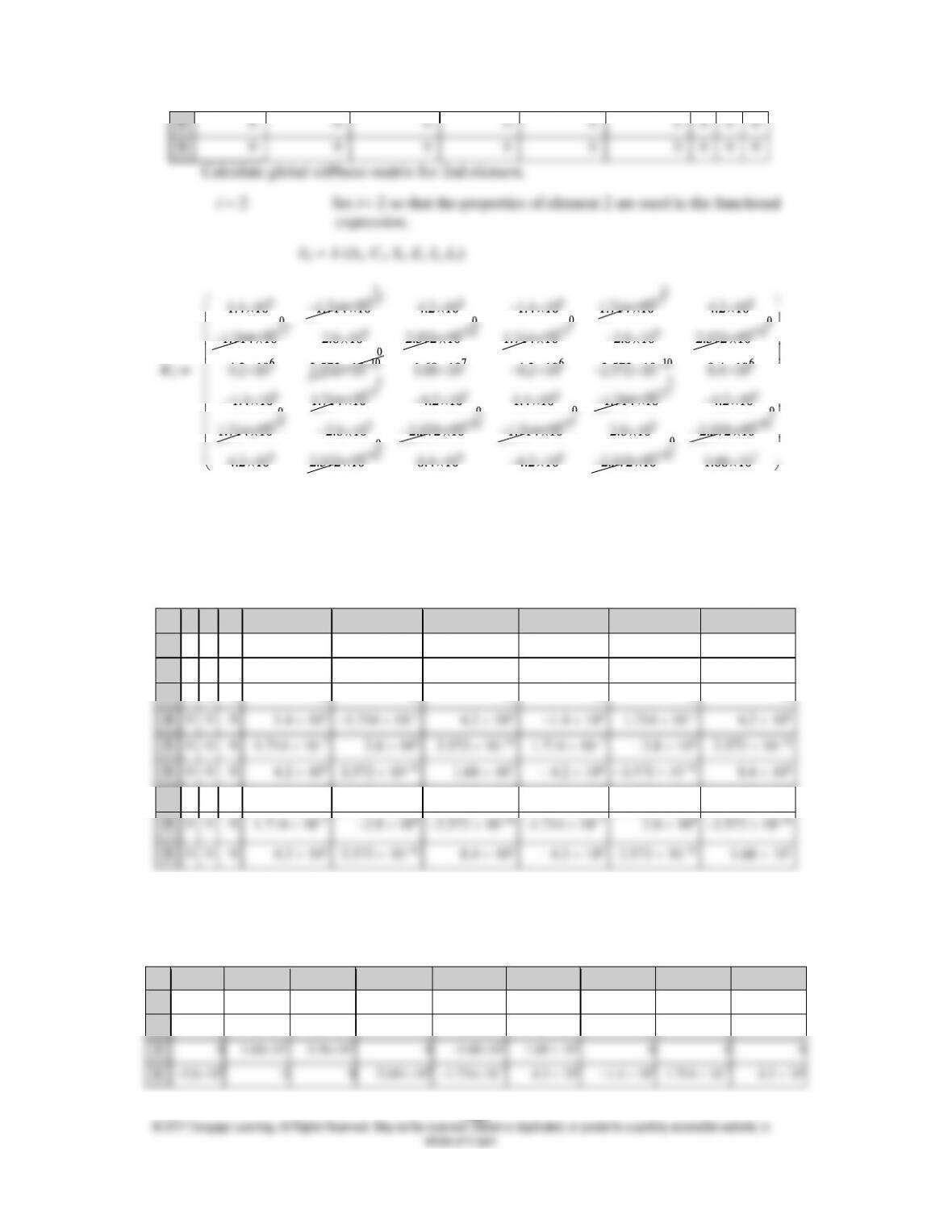
8
0
0
0
0
0
0
0
0
0
9
0
0
0
0
0
0
0
0
0
Calculate global stiffness matrix for 2nd element.
i = 2 Set i = 2 so that the properties of element 2 are used in the functional
expression.
k2 = k (Ai, Ci, Si, E, Ii, Li)
00
67
0
0 0 0
0
0
0
0
00
0
0
0
1.4 10 1.714 10 6 6 7
4.2 10 1.4 10 1.714 10 6
7
4.2 10
1.714 10 9 10
2.8 10 2.572 10 7
1.714 10 9 10
2.8 10 2.572 10
6 10
67
1.4 10 1.714 10 6 6 7
4.2 10 1.4 10 1.714 10 6
7
4.2 10
1.714 10 9 10
2.8 10 2.572 10 7
1.714 10 9 10
2.8 10 2.572 10
6 10
4.2 10 2.572 10 6 6 10
8.4 10 4.2 10 2.572 10 7
1.68 10
Augment element global k matrix with rows and columns of zeros to facilitate the assembly
of the total global stiffness matrix. As before, we need 9 rows and columns.
k2a = augment (ZeroCol,ZeroCol, ZeroCol, k2)
k2b = stack(ZeroRow, ZeroRow, ZeroRow, k2a)
k2b =
0
1
2
3
4
5
6
7
8
9
1
0
0
0
0
0
0
0
0
0
2
0
0
0
0
0
0
0
0
0
3
0
0
0
0
0
0
0
0
0
4
0
0
0
1.4 106
–1.714 10–7
4.2 106
–1.4 106
1.714 10–7
4.2 106
5
0
0
0
–1.714 10–7
2.8 109
2.572 10–10
1.714 10–7
– 2.8 109
2.572 10–10
6
0
0
0
4.2 106
2.572 10–10
1.68 107
– 4.2 106
– 2.572 10–10
8.4 106
7
0
0
0
–1.4 106
1.714 10–7
– 4.2 106
1.4 106
–1.714 10–7
– 4.2 106
8
0
0
0
1.714
–2.8
–2.572
–1.714
2.8
–2.572
9
0
0
0
4.2 106
2.572 10–10
8.4 106
– 4.2 106
– 2.572 10–10
1.68 107
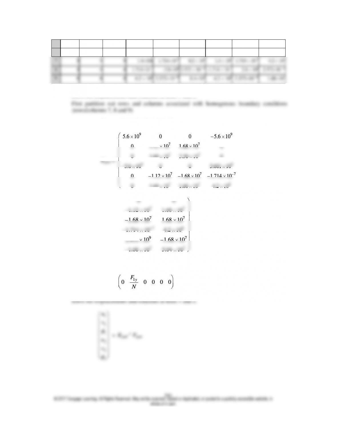
Calculate total global stiffness matrix by adding augmented matrices for each element.
K = k1b + k2b
K =
0
1
2
3
4
5
6
7
8
9
1
5.6109
0
0
–5.6109
0
0
0
0
0
2
0
1.12107
1.68107
0
–1.12107
1.68 107
0
0
0
3
0
1.68107
3.36107
0
–1.68107
1.68 107
0
0
0
4
–5.6109
0
0
5.601109
–1.71410–7
4.2 106
–1.4 106
1.714 10–7
4.2 106
5
0
–1.12107
–1.68107
–1.71410–7
2.811109
–1.68 107
1.714 10–7
– 2.8 109
2.572 10–10
6
0
1.68107
1.68107
4.2106
–1.68107
5.04107
–4.2 106
2.572 10–10
8.4 106
7
0
0
0
–1.4106
1.71410–7
–4.2 106
1.4 106
–1.714 10–7
– 4.2 106
8
0
0
0
1.71410–7
–2.8109
2.572 10–10
–1.714 10–7
2.8 109
2.57210–10
9
0
0
0
4.2 106
2.57210–10
8.4106
–4.2 106
2.57210–10
1.68107
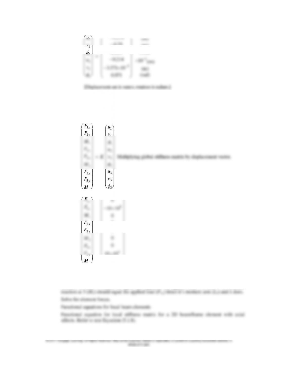
Solve for displacements and rotations at node 1 and 2.
Kpart = submatrix (K, 1, 6, 1, 6)
99
77
77
5.6 10 0 0 5.6 10
0 1.12 10 1.68 10 0
0 1.68 10 3.36 10 0
1
1
1
u
v
0.214 (m)
0.25 (m)
(rad)
0.089