4.6 If the strain history
!
“(s)
0 < s ≤ t, is specified, (3.39a) can be regarded as an
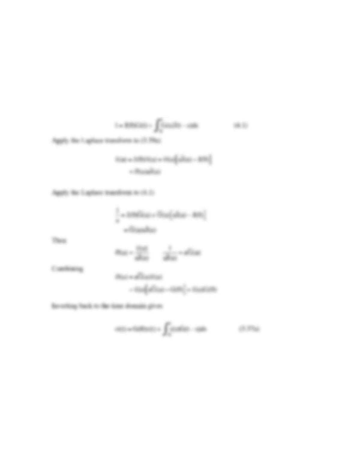
equation for the corresponding stress history. Using the Laplace transform and (4.1) or
(4.2), show that the solution of (3.39a) for the stress history is given by (3.37a).
SOLUTION
“(t) =J(0)#(t) +#(s)˙
J (t $s)ds
0
t
%
(3.39a)
1=J(0)G(t) +G(s)˙
J (t “s)ds
0
t
#
(4.1)
!
4.7 Consider a linear viscoelastic solid whose stress relaxation function has the
form
!
G(t) =0.1+0.9e“t 2
( )
#104N /m2
.
Find the strain history produced when the material is subjected to the following stress
history,
!
“(t) =“o1#e#t c
( )
$104N /m2
.
SOLUTION
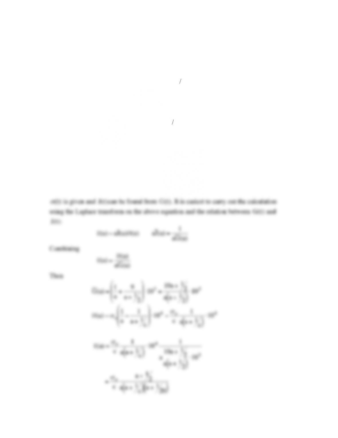
The strain history is calculated from
!
“(t) =#(0)J(t) +J(t $s) ˙
# (s)
0
t
%ds
!
“(t)
is given and
!
J(t)
can be found from
!
G(t)
. It is easiest to carry out the calculation
using the Laplace transform on the above equation and the relation between
!
G(t)
and
!
J(t)
:
!
“ (a) =aJ (a)# (a)
!
aJ (a) =1
aG (a)
Combining
!
“ (a) =# (a)
aG (a)
Then
!
G (a) =1
a+9
a+12
“
#
$
$
%
&
‘
‘
(103=10a +12
a a +12
( )
(103
!
“ (a) =“o
1
a#1
a+1c
$
%
&
&
‘
(
)
)
*104=“o
c
1
a a +1c
( )
*104
!
“ (a) =#o
c
1
a a +1c
( )
$1041
a10a +12
a a +12
( )
$103
!
=“o
c
a+1
2
a a +1
c
( )
a+1
20
( )
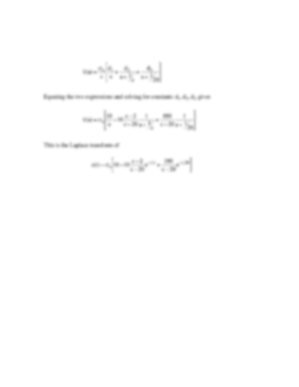
The partial fraction expansion is
!
4.8 If
!
“R
and
!
“C
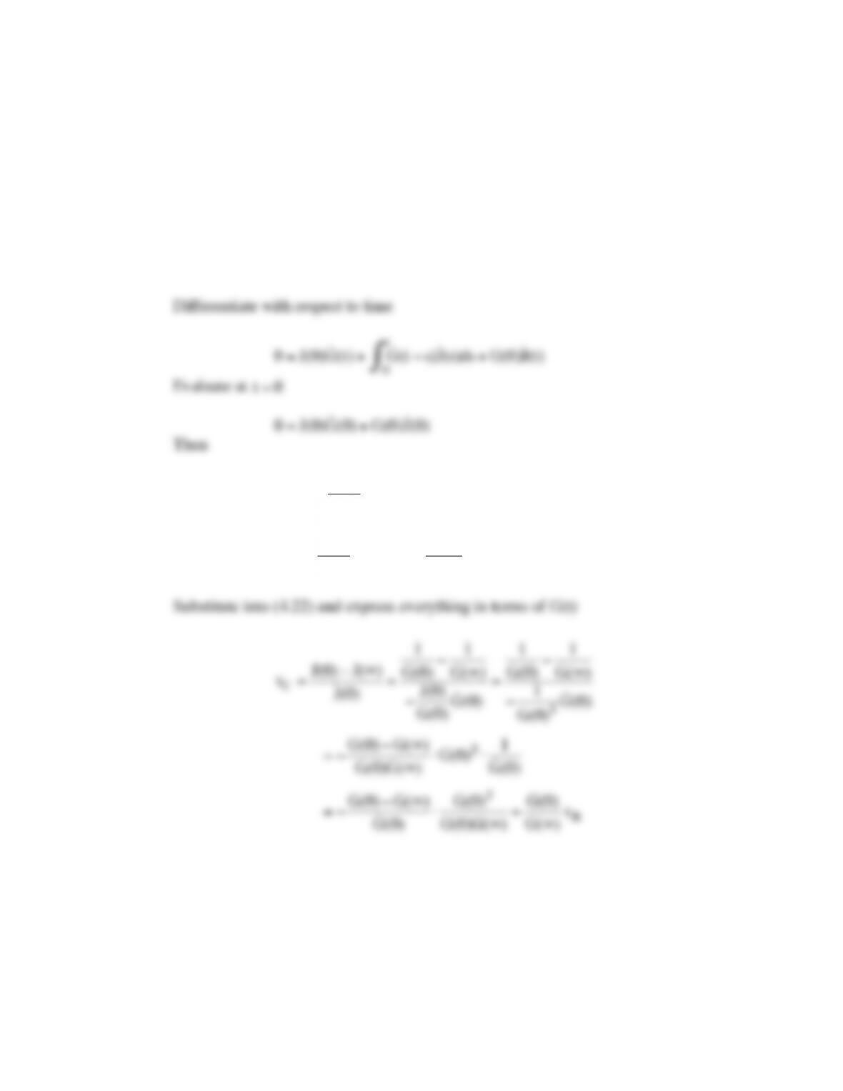
are defined as in (4.22), show that they satisfy (4.24).
Suggestion: Differentiate (4.1) or (4.2) with respect to time and evaluate at
!
t=0
.
SOLUTION
1=J(0)G(t) +G(t “s)˙
J (s)ds
0
t
#
(4.1)
!
!
!
˙
J (0) =“J(0)
G(0)
˙
G (0)
Recall
J(0) =1
G(0)
J(“)=1
G(“)
!
!
!
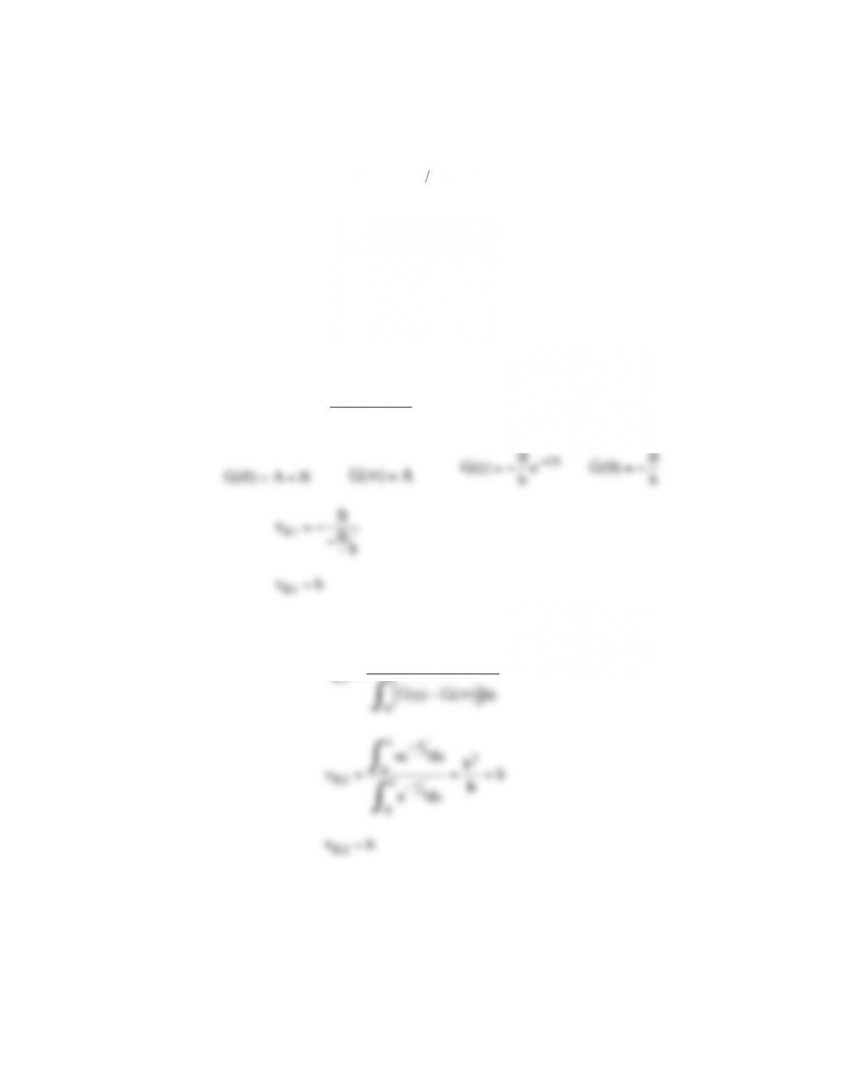
4.9 Consider a relaxation function of the form
!
G(t) =A+Be“t b
,
where A = G(∞) and B = G(0) – G(∞).
(a) Let
!
“R1
be a relaxation time according to Definition 1. Calculate it for this G(t).
(b) Let
!
“R 2
be a relaxation time according to Definition 2. Calculate it for this G(t).
SOLUTION
(a) Definition 1 is
!
“R1 =#G(0) #G($)
˙
G (0)
Then
G(0) =A+B
G(“)=A
˙
G (t) =“B
be“t b
˙
G (0) =“B
b
!
!
“R1 =b
(b) Definition 2 is
!
“R2 =
s G(s) #G($)
[ ]
ds
0
$
%
G(s) #G($)
[ ]
ds
0
$
%
!
“R 2 =
se#s
bds
0
$
%
e#s
bds
0
$
%=b2
b=b
!
“R 2 =b