Chapter 14
14.1
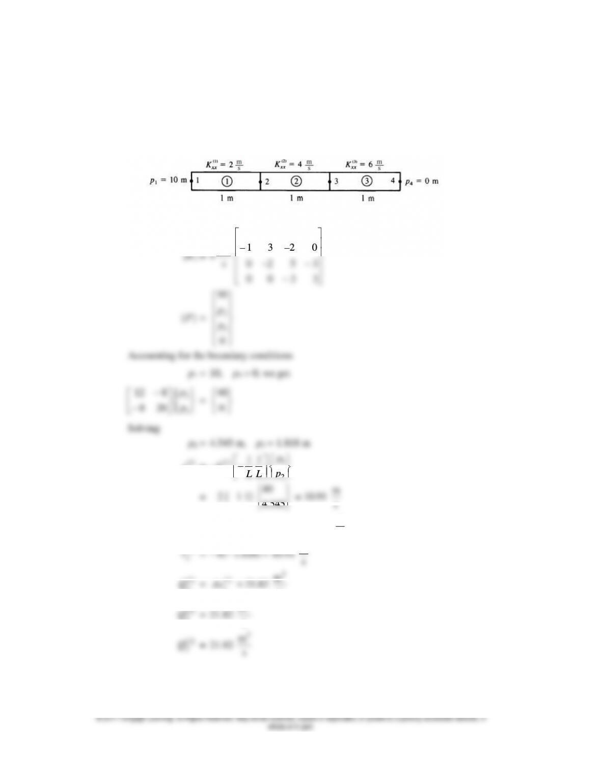
Global [K]
2
m
s
1 – 1 0 0
1 3 2 0
0 2 5 3
0 0 3 3
{P} =
2
3
10
0
p
p
Accounting for the boundary conditions
p1 = 10, p4 = 0, we get
2
3
12 8
8 20
p
p
=
40
0
Solving
p2 = 4.545 m, p3 = 1.818 m
(1)
x
v
= –
1
(1)
2
11
xx
p
kp
LL
40
4.545
m
s
(2)
x
v
= – 4 [– 4.545 + 1.818] = 10.91
m
s
v
(3)
x
m
s
(1)
f
Q
=
(1)
x
Av
= 21.82
3
m
s
(2)
f
Q
= 21.82
3
m
s
(3)
3
m
f
Q
s
540
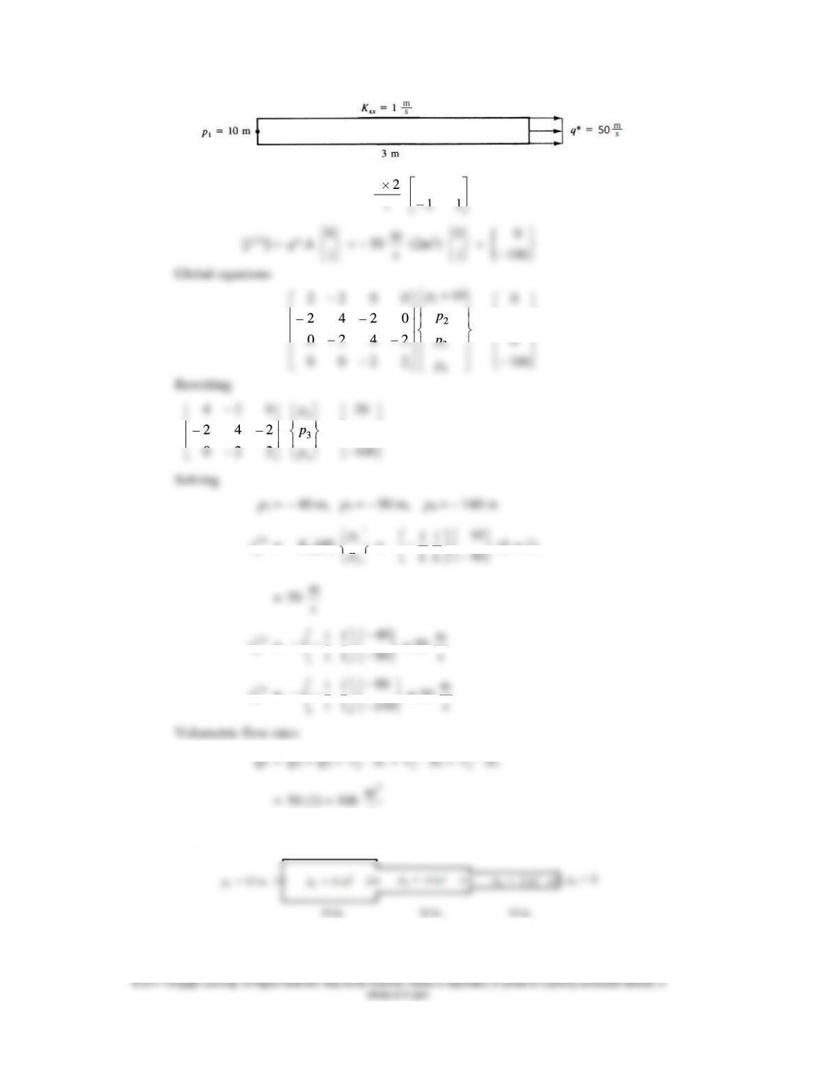
[k(1)] = [k(2)] = [k(3)] =
12
1
1 – 1
– 1 1
s
0
m
0
0
1
2
3
4
= 10
2 2 0 0
2 4 2 0
0 2 4 2
0 0 2 2
p
p
p
p
=
0
0
0
100
4 2 0
242
0 2 2
2
3
4
p
p
p
=
20
0
100
(1)
x
v
= – Kxx[B]
1
2
p
p
= –
10
11
40
LL
(L = 1)
m
s
(2)
x
v
=
40
11
190
11
= 50
m
s
(3)
x
v
=
90
11
1140
11
= 50
m
s
x
x
x
3
m
s
14.3
541
11
11
[k(2)] = 0.4
11
11
[k(3)] = 0.2
11
11
2
3
4
10 in.
0.6 – 0.6 0 0
–0.6 1.0 0.4 0
0 0.4 0.6 0.2
=0
0 0 0.2 0.2
p
p
p
=
0
0
0
0
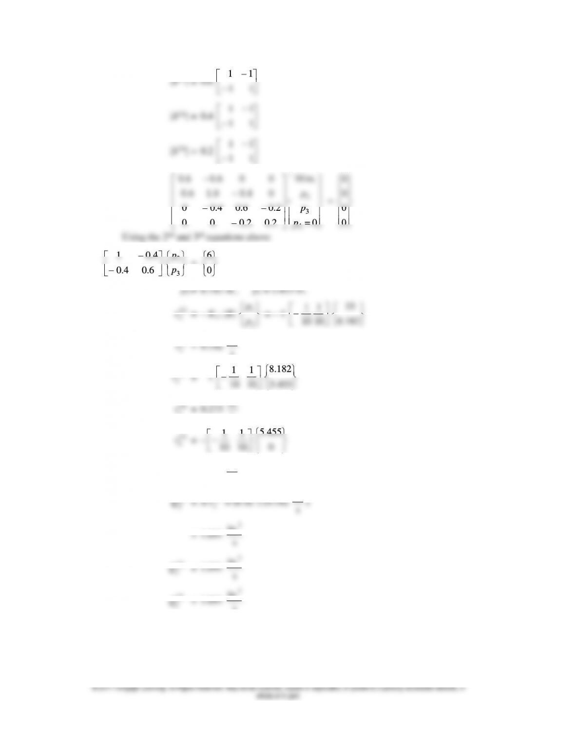
Using the 2nd and 3rd equations above
1 0.4
0.4 0.6
2
3
p
p
=
6
0
(1)
x
2
p
10 10
8.182
s
(2)
v
(1)
in.
x
10 10
5.455
(2)
x
v
= 0.273
in.
s
v
(3)
x
11
10 10
5.455
0
= 0.545
in.
s
(1)
f
(1)
x
in.
s
s
3
in.
3
in.
f
s
3
in.
f
s
14.4
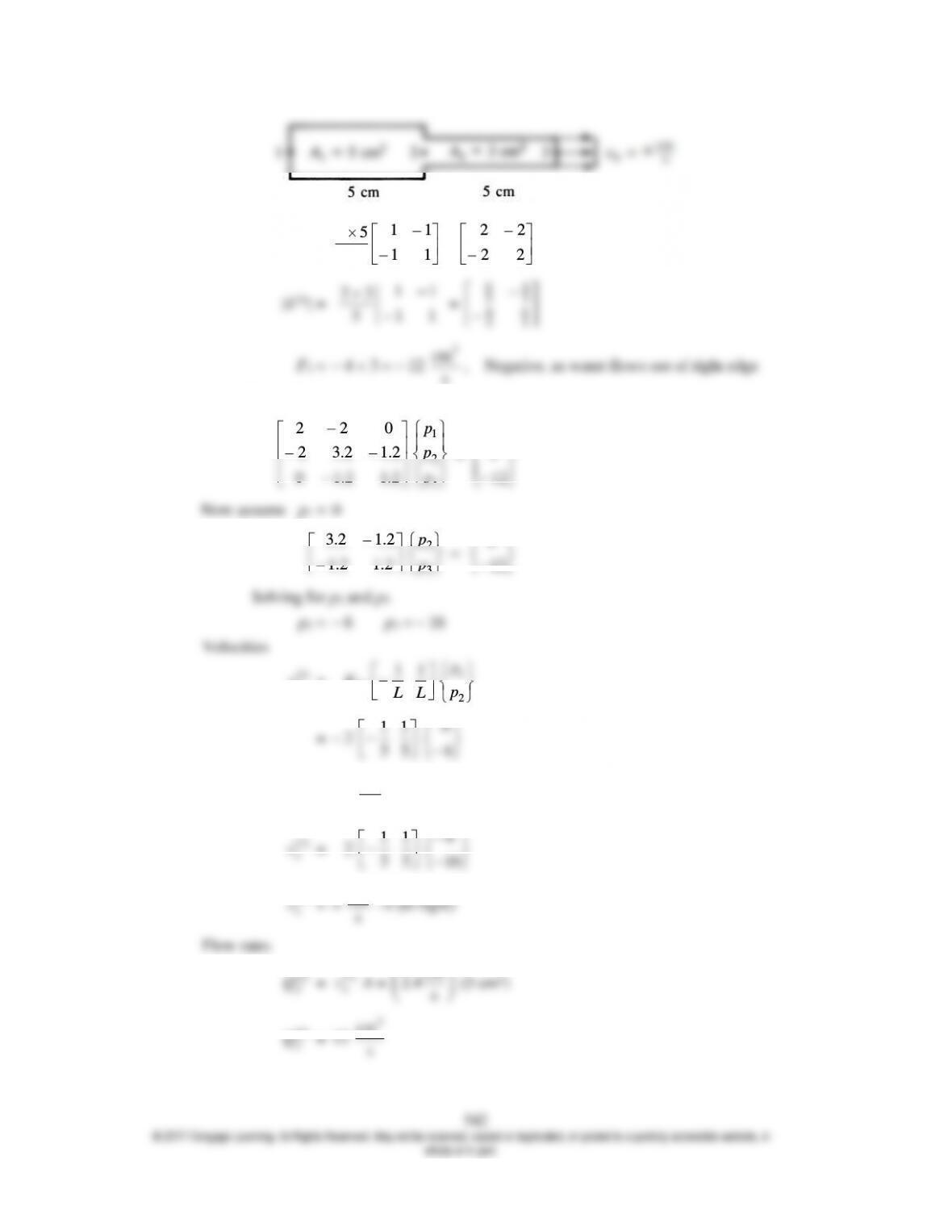
[k(1)] =
11
25
11
5
=
22
22
11
23
66
55
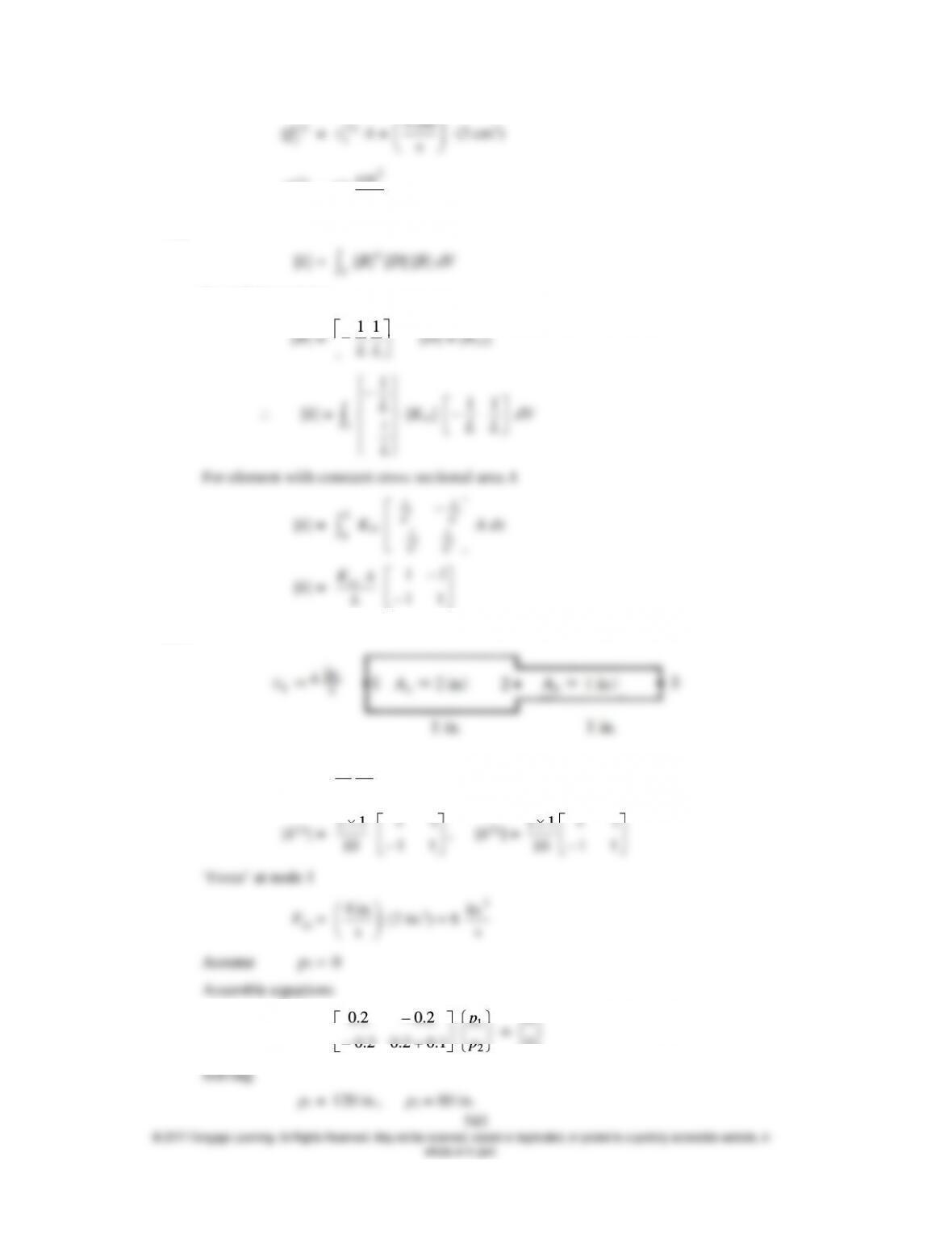
Q
(2)
f
(2)
x
4 cm
s
(2)
f
Q
= 12
3
cm
s
14.5
V
For 1-D formulation
11
LL
[k] =
v
1
1
L
L
[Kxx]
11
LL
dV
For element with constant cross sectional area A
[k] =
0
L
Kxx
22
22
11
11
LL
LL
A dx
[k] =
xx
KA
L
11
11
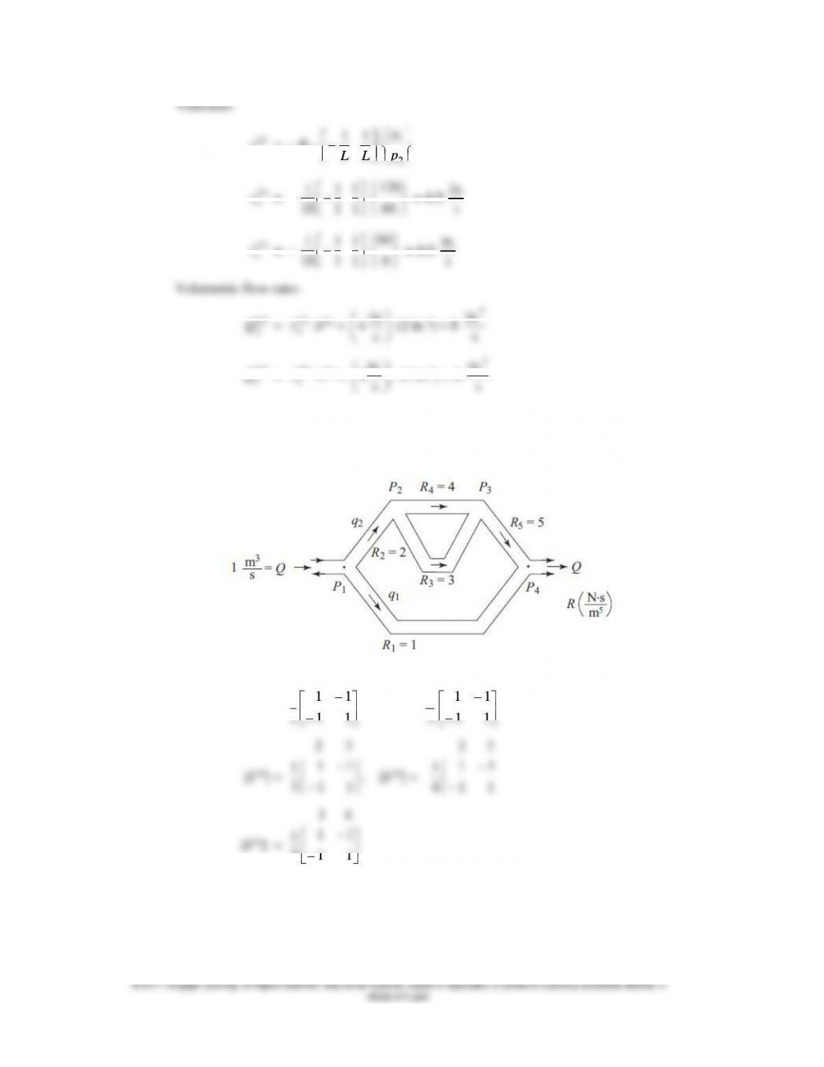
14.6
Kxx =
1 in.
10 s
21
1 – 1
1 – 1
11
(1)
x
v
= – Kxx
11
LL
1
2
p
p
(1)
1 1 1
120
in.
v
1 1 1
in.
(1)
x
v
11
22
1 1 1 1 1 1
2 2 3 4 2 4
11 111
10
1
2
p
p
1
1
0
Q
11
1
11
10
11
20
2 3 2 3
11
1
11
30
11
1
11
40
3 4
[k(5)] =
11
1
11
50
Assemble
1 2 3
1 1 1
10 20 20
1 1 1 1 1 1
20 20 30 40 30 40
1 1 1 1 1
30 40 30 40 50
5
–0
in.
lb s
1
2
3
2
lb
in.
p
p
3
1000
0
in.
s
Solve for p1, p2, p3 using Mathcad as
p1 = 8971 psi, p2 = 6912 psi, p3 = 5147 psi,
14
=0PP
1 2
––P P
23
PP
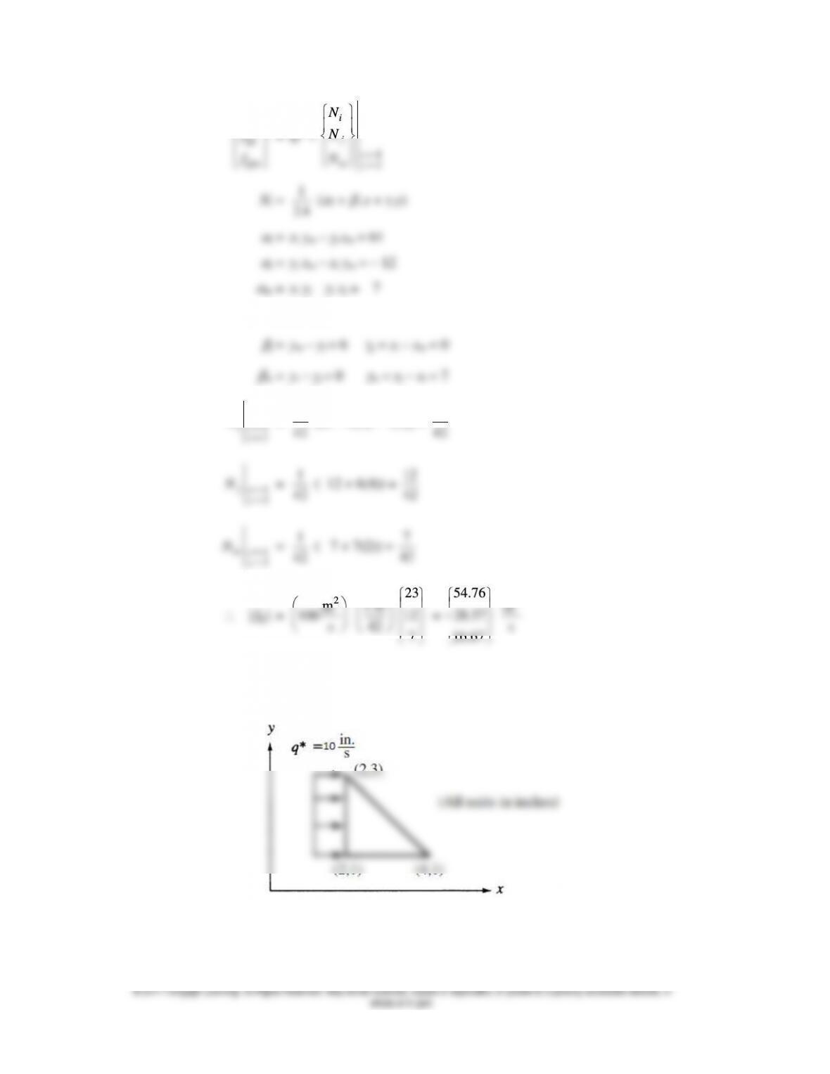
547
Qi
Qj
Qm
f
f
4
2
i
j
x
my
N
N
Ni =
1
2A
(
i +
i x +
i
y)
i = xi ym – yj xm = 61
j = yj xm – xi ym = – 12
m = xi yj – yi xj = – 7
i = yi – ym = – 6 i = xm – xj = – 7
=4
=2
ix
y
N
=
1
42
(61 – 6(4) – 7(2)) =
23
42
=4
=2
jx
y
1
42
12
42
=4
=2
mx
y
N
=
1
42
(– 7 + 7(2)) =
7
42
{fQ} =
2
m
100 s
1 m
42
23
12
7
=
54.76
28.57
16.67
3
m
s
14.9
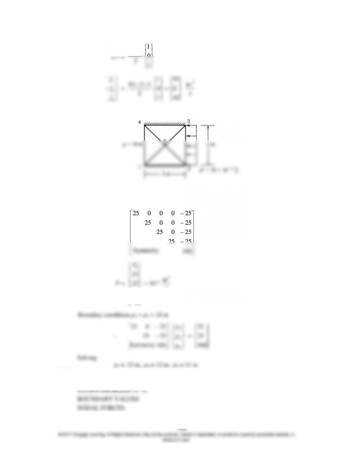
1
*0
q Lt
2
3
f
2
1 10
s
14.10
From Equations (14.3.16)
[K] =
25 0 0 0 25
25 0 0 25
25 0 25
25 25
Symmetry 100
10–5
1
25
F
3
m
LOADING CASE 2
1 0.50000E+04
*PRESCRIBED NODAL VALUES*
26 0.50000E+03
27 0.50000E+03
28 0.50000E+03
FLUIDS PROBLEM 14–11
NODAL VALUES, LOADING CASE 1
1 – 0.46404E+03 2 0.37597E+02
5 0.14359E+07 6 – 0.26094E+03
9 0.45441E+02 10 0.25835E+03
NODAL VALUES, LOADING CASE 2
1 – 0.49446E+03 2 0.23005E+02
5 0.14476E+07 6 – 0.28970E+03
9 0.30588E+02 10 0.25067E+03