Mathematics Chapter 9 Equating this to the right hand side of the second

Solutions — Chapter 9

9.1.1.

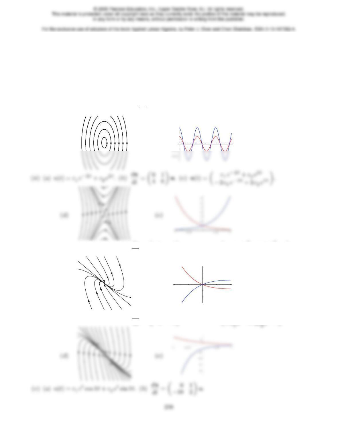
(i) (a)u(t) = c1cos 2t+c2sin 2t. (b)du

dt = 0 1

−4 0 !u. (c)u(t) = c1cos 2t+c2sin 2t

−2c1sin 2t+ 2c2cos 2t!.

(d)(e)

246 8

0.2

0.4

(iii ) (a)u(t) = c1e−t+c2te−t. (b)du

dt = 0 1

−1−2!u. (c)u(t) = c1e−t+c2te−t

(c2−c1)e−t−c2te−t!.

(d)(e)

-1 -0.5 0.5 1

-3

-2

-1

1

2

3

(iv ) (a)u(t) = c1e−t+c2e−3t. (b)du

dt = 0 1

−3−4!u. (c)u(t) = c1e−t+c2e−3t

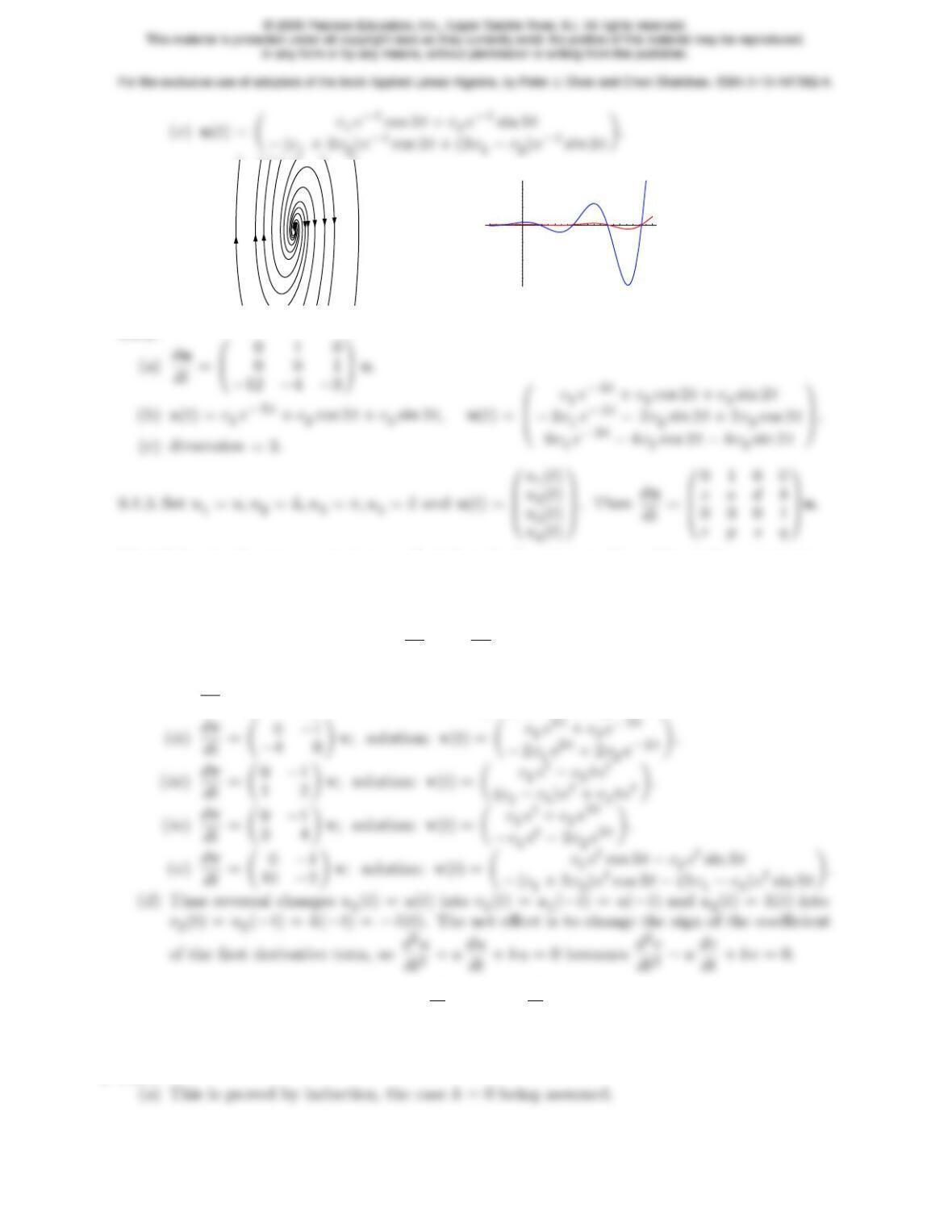
(d)(e)

-1 1 2 3 4

-30

-20

-10

10

20

9.1.2.

9.1.4. False; by direct computation, we find that the functions u1(t), u2(t) satisfy a quadratic

equation αu2

1+β u1u2+γ u2

2+δu1+εu2=cif and only if c1=c2= 0.

♦9.1.5.

(a) Use the chain rule to compute dv

dt =−du

dt (−t) = −Au(−t) = −Av.

(b) Since v(t) = u(−t) parametrizes the same curve as u(t), but in the reverse direction.

(c) (i)dv

dt = 0−1

4 0 !v; solution: v(t) = c1cos 2t−c2sin 2t

2c1sin 2t+ 2c2cos 2t!.

9.1.6. (a) Use the chain rule to compute d

dt v(t) = 2 d

dt u(2t) = 2Au(2t) = 2 Av(t),and

so the coefficient matrix is multiplied by 2. (b) The solution trajectories are the same, but

the solution moves twice as fast (in the same direction) along them.

♦9.1.7.

239

9.1.8. False. If ¦

u=Authen the speed along the trajectory at the point u(t) is kAu(t)k.

So the speed is constant only if kAu(t)kis constant. (Later, in Lemma 9.31, this will be

shown to correspond to Abeing a skew-symmetric matrix.)

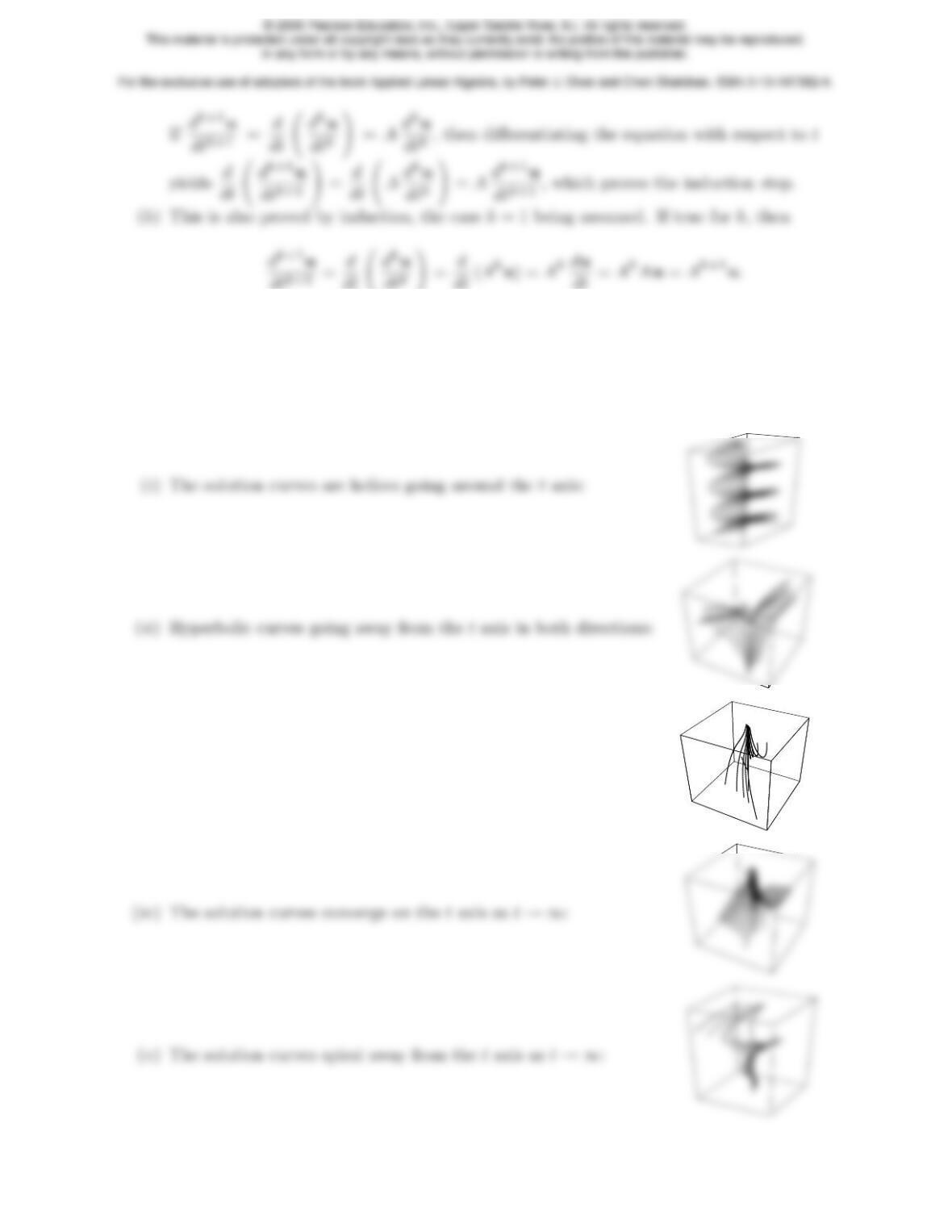
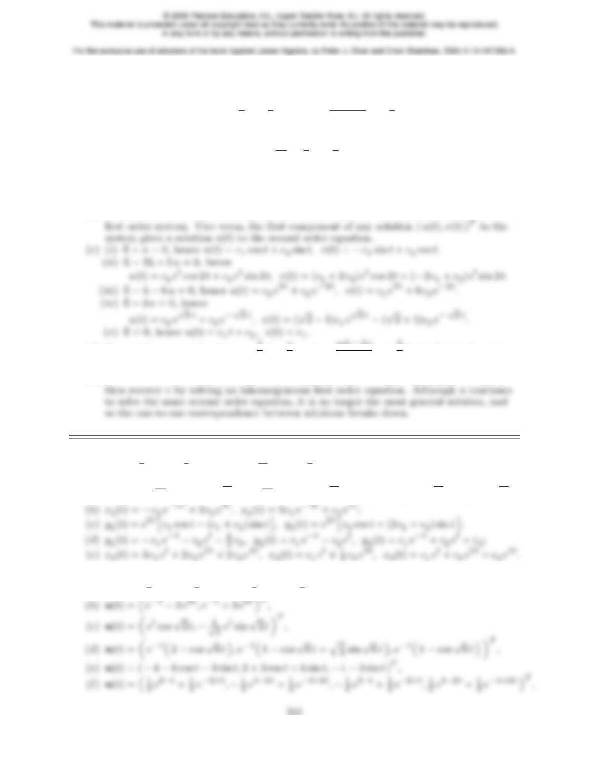
♠9.1.9. In all cases, the taxis is plotted vertically, and the three-dimensional solution curves

(u(t),¦

u(t), t)Tproject to the phase plane trajectories (u(t),¦

u(t))T.

(iii ) The solution curves converge on the taxis as t→ ∞:

240

♥9.1.10.

(a) Assuming b6= 0, we have

v=1

b

¦

u−a

bu, ¦

v=bc −ad

bu+d

b

¦

u.(∗)

Differentiating the first equation yields

dv

dt =1

b

¦¦

u−a

b

¦

u.

Equating this to the right hand side of the second equation yields leading to the second

order differential equation

¦¦

u−(a+d)¦

u+ (ad −bc)u= 0.(∗∗)

(b) If u(t) solves (∗∗), then defining v(t) by the first equation in (∗) yields a solution to the

(d) For c6= 0 we can solve for u=1

d

¦

v−c

dv, ¦

u=ad −bc

du+b

d

¦

v,leading to the same

second order equation for v, namely, ¦¦

v−(a+d)¦

v+ (ad −bc)v= 0.

(e) If b= 0 then usolves a first order linear equation; once we solve the equation, we can

9.1.11. u(t) = 7

5e−5t+8

5e5t, v(t) = −14

5e−5t+4

5e5t.

9.1.12.

(a)u1(t) = (√10−1)c1e(2+√10) t−(√10+1)c2e(2−√10) t, u2(t) = c1e(2+√10) t+c2e(2−√10) t;

9.1.13.

(a)u(t) = “1

2e2−2t+1

2e−2+2 t,−1

2e2−2t+1

2e−2+2 t”T,

9.1.14. (a)x(t) = e−tcos t, y(t) = −e−tsin t; (b)

9.1.17. The coefficient matrix has eigenvalues λ1=−5, λ2=−7,and, since the coefficient ma-

trix is symmetric, orthogonal eigenvectors v1= 1

1!,v2= −1

1!.The general solution

is

u(t) = c1e−5t 1

1!+c2e−7t −1

1!.

For the initial conditions

9.1.18.

(a) Eigenvalues: λ1= 0, λ2= 1, λ3= 3, eigenvectors: v1=0

B

@

1

11

C

A,v2=0

B

@

1

0

−11

C

A,v3=0

B

@

1

−2

11

C

A.

(b) By direct computation, v1·v2=v1·v3=v2·v3= 0.

242

9.1.19. The general complex solution to the system is

u(t) = c1e−t0

B

@−1

1

11

C

A+c2e(1+2 i ) t0

B

@

1

i

11

C

A+c3e(1−2i)t0

B

@

1

−i

11

C

A.

Substituting into the initial conditions,

9.1.20. Only (d) and (g) are linearly dependent.

♦9.1.21. Using the chain rule, d

dt e

u(t) = du

dt (t−t0) = Au(t−t0) = Ae

u(t), and hence e

u(t) solves

the differential equation. Moreover, e

u(t0) = u(0) = bhas the correct initial conditions.

The trajectories are the same curves, but e

u(t) is always ahead of u(t) by an amount t0.

9.1.24. dv

dt =Sdu

dt =S Au=S AS−1v=Bv.

♦9.1.25.

(i) This is an immediate consequence of the preceding two exercises.

(ii ) (a)u(t) = −1 1

1 1 ! c1e−2t

c2e2t!, (b)u(t) = −1 1

1 1 ! c1e3t

c2e−t!,

243

9.1.26.

(a) c1e2t+c2t e2t

c2e2t!, (b)0

@c1e−t+c2“1

3+t”e−t

3c1e−t+ 3c2te−t1

A,

B

c1e−t+c2et+c3t et

1

C

9.1.27. (a)du

dt = 2−1

2

0 1 !u, (b)du

dt = −1 1

−9−1!u, (c)du

dt = 0 0

1 0 !u,

9.1.28. (a) No, since neither dui

dt is a linear combination of u1,u2. Or note that the trajec-

tories described by the solutions cross, violating uniqueness. (b) No, since polynomial solu-

tions a two-dimensional system can be at most first order in t. (c) No, since a two-dimensional

system has at most 2 linearly independent solutions. (d) Yes: ¦

u= −1 0

0 1 !u. (e) Yes:

244

values of the coefficient matrix are −3,±2 i with eigenvectors 0

B

@

1

−3

91

C

A,0

B

@

1

±2 i

−41

C

Aand the

resulting solution is u(t) = 0

B

@

c1e−3t+c2cos 2t+c3sin 2t

−3c1e−3t−2c2sin 2t+ 2c3cos 2t

9c1e−3t−4c2cos 2t−4c3sin 2t

1

C

A, which is the same as

that found in Exercise 9.1.2.

9.1.31. The degree is at most n−1, and this occurs if and only if Ahas only one Jordan chain

in its Jordan basis.

♦9.1.32.

(a) By direct computation,

9.1.33.

(a) The equilibrium solution satisfies Au⋆=−b, and so v(t) = u(t)−u⋆satisfies ¦

v=¦

u=

Au+b=A(u−u⋆) = Av, which is the homogeneous system.

9.2.1.

(a) Asymptotically stable: the eigenvalues are −2±i ;

245

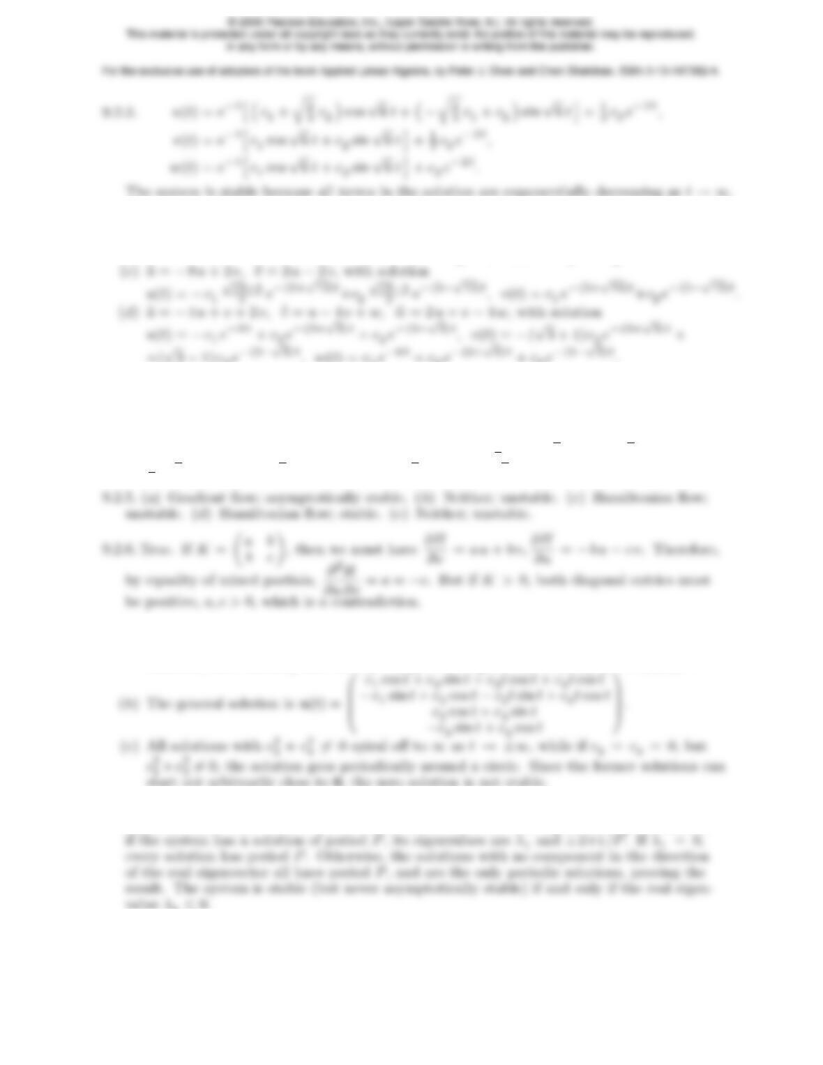
9.2.3.

(a)¦

u=−2u, ¦

v=−2v, with solution u(t) = c1e−2t, v(t) = c2e−2t.

(b)¦

u=−v, ¦

v=−u, with solution u(t) = c1et+c2e−t, v(t) = −c1et+c2e−t.

9.2.4.

(a)¦

u= 2v, ¦

v=−2u, with solution u(t) = c1cos 2t+c2sin 2t, v(t) = −c1sin 2t+c2cos 2t;

stable.

(b)¦

u=u, ¦

v=−v, with solution u(t) = c1et, v(t) = c2e−t; unstable.

(c)¦

u=−2u+ 2v, ¦

v=−8u+ 2v, with solution u(t) = 1

4(c1−√3c2) cos 2√3t+

1

4(√3c1+c2) sin 2√3t, v(t) = c1cos 2√3t+c2sin 2√3t; stable.

9.2.7.

(a) The characteristic equation is λ4+ 2λ2+ 1 = 0, and so ±i are double eigenvalues.

However, each has only one linearly independent eigenvector, namely ( 1,±i,0,0 )T.

9.2.8. Every solution to a real first order system of period Pcomes from complex conjugate

eigenvalues ±2πi/P . A 3 ×3 real matrix has at least one real eigenvalue λ1. Therefore,

9.2.9. No, since a 4 ×4 matrix could have two distinct complex conjugate pairs of purely imag-

inary eigenvalues, ±2πi/P1,±2πi/P2, and would then have periodic solutions of periods

246

9.2.10. The system is stable since ±i must be simple eigenvalues. Indeed, any 5 ×5 matrix has

5 eigenvalues, counting multiplicities, and the multiplicities of complex conjugate eigenval-

9.2.11. True, since Hn>0 by Proposition 3.34.

9.2.12. True, because the eigenvalues of the coefficient matrix −Kare real and non-negative,

λ≤0. Moreover, as it is symmetric, all its eigenvalues, including 0, are complete.

9.2.13. (a)¦

v=Bv=−Av. (b) True, since the eigenvalues of B=−Aare minus the

eigenvalues of A, and so will all have positive real parts. (c) False. For example, a saddle

9.2.14. The eigenvalues of −A2are all of the form −λ2≤0, where λis an eigenvalue of A.

Thus, if Ais nonsingular, the result is true, while if Ais singular, then the equilibrium so-

lutions are stable, since the 0 eigenvalue is complete, but not asymptotically stable.

9.2.15. (a) True, since the sum of the eigenvalues equals the trace, so at least one must be

9.2.16.

(a) Every v∈ker Kgives an equilibrium solution u(t)≡v.

(b) Since Kis complete, the general solution has the form

9.2.17.

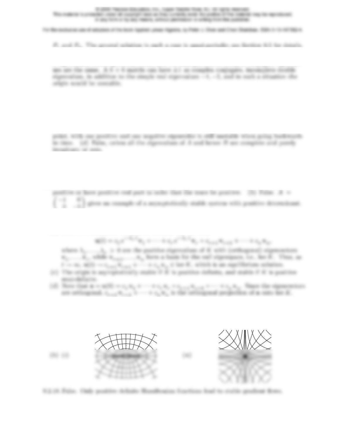
(a) The tangent to the Hamiltonian trajectory at a point ( u, v )Tis v= ( ∂H/∂v, −∂H/∂u )T

while the tangent to the gradient ﬂow trajectory is w= ( ∂H/∂u, ∂H/∂v )T. Since

v·w= 0, the tangents are orthogonal.

0.5

1

0.5

0.75

1

247

9.2.19.

(a) When q(u) = 1

2uTKuthen

♥9.2.20.

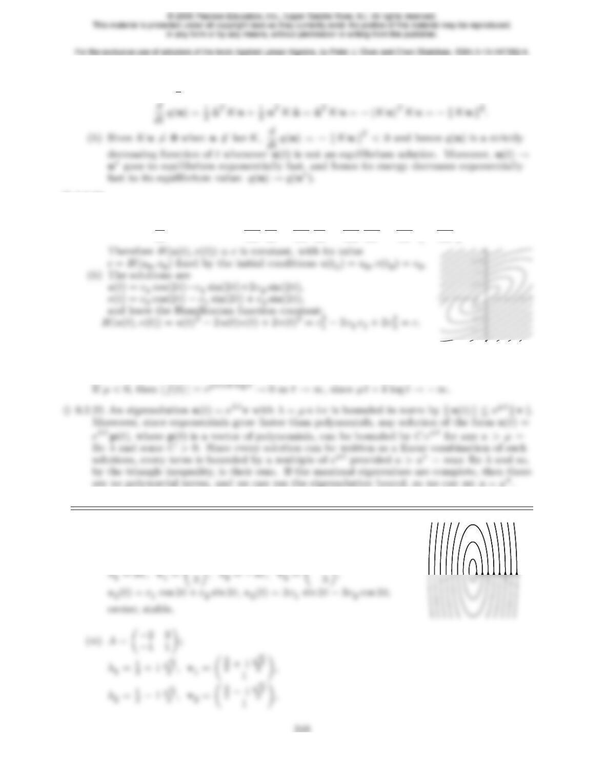
(a) By the multivariable calculus chain rule

d

dt H(u(t), v(t)) = ∂H

∂u

du

dt +∂H

∂v

dv

dt =∂H

∂u

∂H

∂v +∂H

∂v −∂H

∂u !≡0.

-1

♦9.2.21. In both cases, |f(t)|=tkeµ t. If µ > 0, then eµ t → ∞, while tk≥1 as t→ ∞, and so

|f(t)| ≥ eµ t → ∞. If µ= 0, then |f(t)|= 1 when k= 0, while |f(t)|=tk→ ∞ if k > 0.

9.3.1.

(i)A= 0−1

9 0 !;

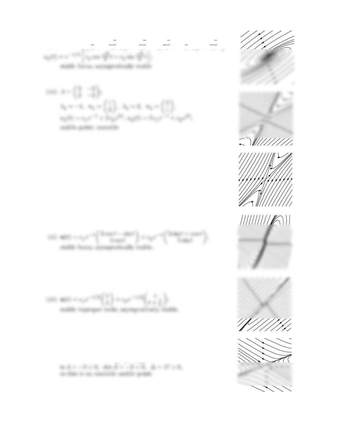
u1(t) = e−t/2»„3

2c1−√3

2c2«cos √3

2t+„√3

2c1+3

2c2«sin √3

2t–,

9.3.2.

(i)u(t) = c1e−t 1

3!+c2et 1

1!;

saddle point; unstable.

9.3.3.

(a) For the matrix A= −1 4

1−2!,

249

This material is protected under all copyright laws as they currently exist. No portion of this material may be reproduced,

in any form or by any means, without permission in writing from the publisher.

For the exclusive use of adopters of the book Applied Linear Algebra, by Peter J. Olver and Cheri Shakiban. ISBN 0-13-147382-4.

(c) For the matrix A= 5 4

1 2 !,

tr A= 7 >0, det A= 6 >0, ∆ = 25 >0,

so this is an unstable node.

(d) (e)

♦9.3.6. For (9.31), the complex solution

eλ tv=e(µ+ i ν)t(w+ i z) = eµ thcos(ν t)w−sin(ν t)zi+eµ thsin(ν t)w+ cos(ν t)zi

leads to the general real solution

u(t) = c1eµ thcos(ν t)w−sin(ν t)zi+c2eµ thsin(ν t)w+ cos(ν t)zi

9.4.1.

(a)0

@

4

3et−1

3e−2t−1

3et+1

3e−2t

4

3et−4

3e−2t−1

3et+4

3e−2t1

A, (b)0

@

1

2et+1

2e−t1

2et−1

2e−t

1

2et−1

2e−t1

2et+1

2e−t1

A= cosh tsinh t

sinh tcosh t!,

9.4.2.

(a)0

B

@

1 0 0

2 sin tcos tsin t

2 cos t−2−sin tcos t1

C

A,

(b)0

B

@

1

6et+1

2e3t+1

3e4t1

3et−1

3e4t1

6et−1

2e3t+1

3e4t

1

3et−1

3e4t2

3et+1

3e4t1

3et−1

3e4t

1

6et−1

2e3t+1

3e4t1

3et−1

3e4t1

6et+1

2e3t+1

3e4t

1

C

A,

251

9.4.3. 9.4.1 (a) det et A =e−t=ettr A, (b) det et A = 1 = ettr A, (c) det et A = 1 = ettr A,

(d) det et A = 1 = ettr A, (e) det et A =e4t=ettr A, (f) det et A =e−2t=ettr A.

9.4.2 (a) det et A = 1 = ettr A, (b) det et A =e8t=ettr A, (c) det et A =e−4t=ettr A,

(d) det et A = 1 = ettr A.

9−2

9cos 3 + 2

3sin 3 2

9−2

9cos 3 −2

3sin 3 1

9+8

9cos 3

9.4.5.

(a)u(t) = cos t−sin t

sin tcos t! 1

−2!= cos t+ 2 sin t

sin t−2 cos t!,

9.4.6. etO= I for all t.

9.4.7. There are none, since et A is always invertible.

♦9.4.10. Assuming Ais an n×nmatrix, since et A is a matrix solution, each of its nindividual

columns must be solutions. Moreover, the columns are linearly independent since e0A= I

is nonsingular. Therefore, they form a basis for the n-dimensional solution space.

9.4.11. (a) False, unless A−1=−A. (b) True, since Aand A−1commute.

252

9.4.13. Set U(t) = A et A, V (t) = et A A. Then, by the matrix Leibniz formula (9.40),

¦

U=

A2et A =A U,

¦

V=A et A A=A V , while U(0) = A=V(0). Thus U(t) and V(t) solve the

same initial value problem, hence, by uniqueness, U(t) = V(t) for all t. Alternatively, one

can use the power series formula (9.46): A et A =∞

X

n= 0

tn

n!An+1 =et AA.

♦9.4.16. First note that An=S BnS−1. Therefore, using (9.46),

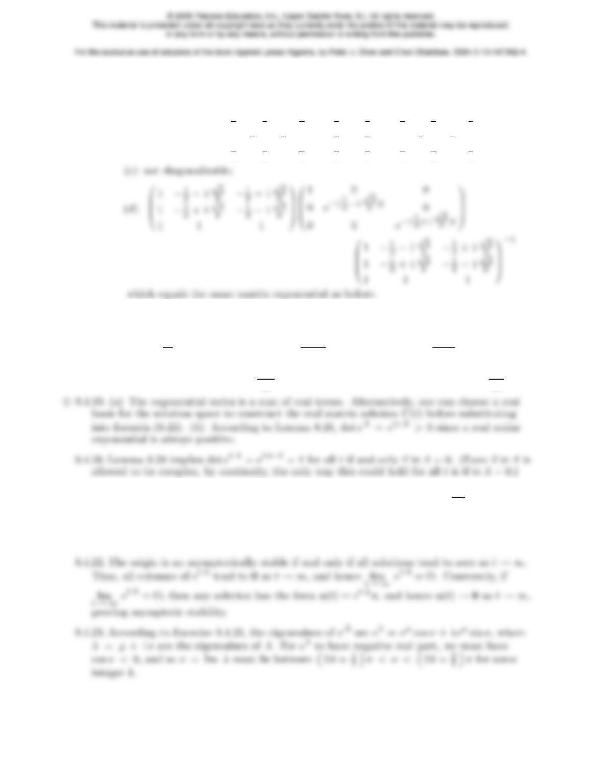
(c) 9.4.1: (a) 1 1

1 4 ! et0

0e−2t! 1 1

1 4 !−1

=0

@

4

3et−1

3e−2t−1

3et+1

3e−2t

4

3et−4

3e−2t−1

3et+4

3e−2t1

A;

(b) 1−1

1 1 ! et0

0e−t! 1−1

1 1 !−1

=0

@

1

2et+1

2e−t1

2et−1

2e−t

1

2et−1

2e−t1

2et+1

2e−t1

A;

253

(b)0

B

@

1−1 1

2 0 −1

1 1 1 1

C

A0

B

@

et0 0

0e3t0

0 0 e4t1

C

A0

B

@

1−1 1

2 0 −1

1 1 1 1

C

A

−1

=0

B

@

1

6et+1

2e3t+1

3e4t1

3et−1

3e4t1

6et−1

2e3t+1

3e4t

1

3et−1

3e4t2

3et+1

3e4t1

3et−1

3e4t

1

6et−1

2e3t+1

3e4t1

3et−1

3e4t1

6et+1

2e3t+1

3e4t

1

C

A;

♦9.4.18. Let Mhave size p×qand Nhave size q×r. The derivative of the (i, j) entry of the

product matrix M(t)N(t) is

d

dt

q

X

k= 1

mik(t)nkj (t) =

q

X

k= 1

dmik

dt nkj (t) +

q

X

k= 1

mik(t)dnkj

dt .

The first sum is the (i, j) entry of dM

dt Nwhile the second is the (i, j) entry of MdN

dt .

♦9.4.21. Let u(t) = et λ vwhere vis the corresponding eigenvector of A. Then, du

dt =λ et λ v=

λu=Au, and hence, by (9.41), u(t) = et A u(0) = et A v. Therefore, equating the two

formulas for u(t), we conclude that et A v=et λ v, which proves that vis an eigenvector of

et A with eigenvalue et λ.

254

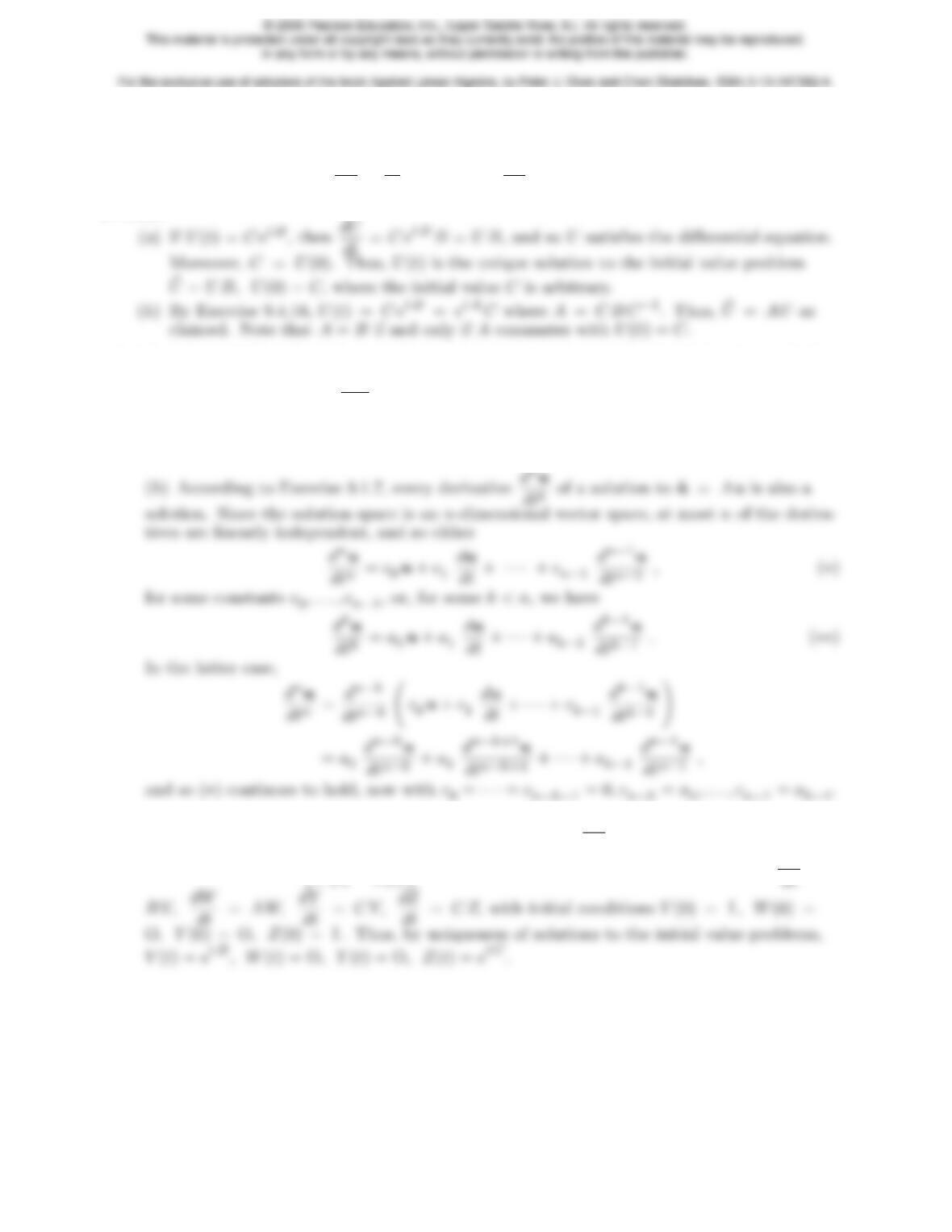
9.4.24. Indeed, the columns of e

U(t) are linear combinations of the columns of U(t), and hence

automatically solutions to the linear system. Alternatively, we can prove this directly using

the Leibniz rule (9.40): de

U

dt =d

dt “U(t)C”=dU

dt C=A U C =Ae

U, since Cis constant.

♦9.4.25.

9.4.26. (a) Let U(t) = ( u1(t). . . un(t) ) be the corresponding matrix-valued function with the

indicated columns. Then duj

dt =

n

X

i= 1

bij uifor all j= 1, . . . , n, if and only if

¦

U=U B

where Bis the n×nmatrix with entries bij . Therefore, by Exercise 9.4.25,

¦

U=AU, where

A=C B C−1with C=U(0).

9.4.27. Write the matrix solution to the initial value problem dU

dt =A U, U(0) = I ,in block

form U(t) = et A = V(t)W(t)

Y(t)Z(t)!. Then the differential equation decouples into dV

255

♦9.4.28.

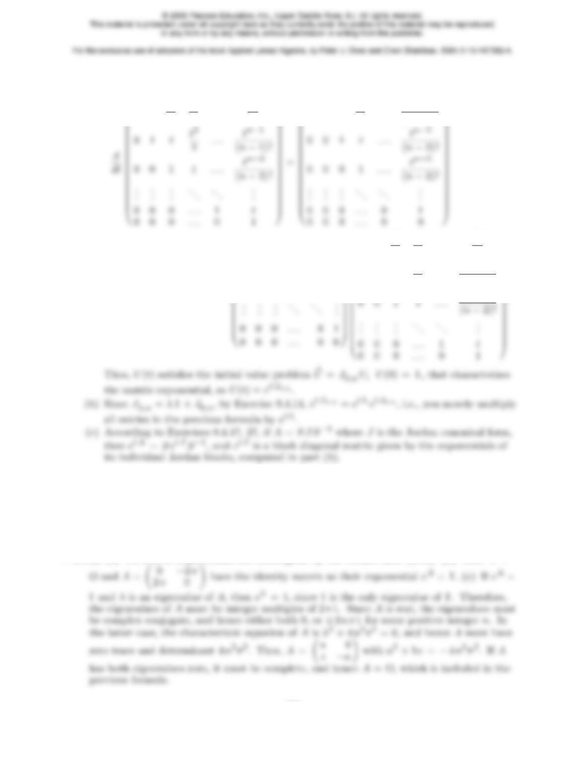
(a)

0

B

1tt2

2

t3

6… tn

n!

1

C

0

B

0 1 tt2

2… tn−1

(n−1)!

1

C

=

0

B

0 1 0 0 … 0

0 0 1 0 … 0

.

..

.

..

.

..

.

.....

.

1

C

0

B

1tt2

2

t3

6. . . tn

n!

0 1 tt2

2. . . tn−1

(n−1)!

1

C

,

♦9.4.29. If Jis a Jordan matrix, then, by the arguments in Exercise 9.4.28, et J is upper triangu-

lar with diagonal entries given by et λ where λis the eigenvalue appearing on the diagonal

of the corresponding Jordan block of A. In particular, the multiplicity of λ, which is the

number of times it appears on the diagonal of J, is the same as the multiplicity of et λ for

et J . Moreover, since et A is similar to et J , its eigenvalues are the same, and of the same

multiplicities.

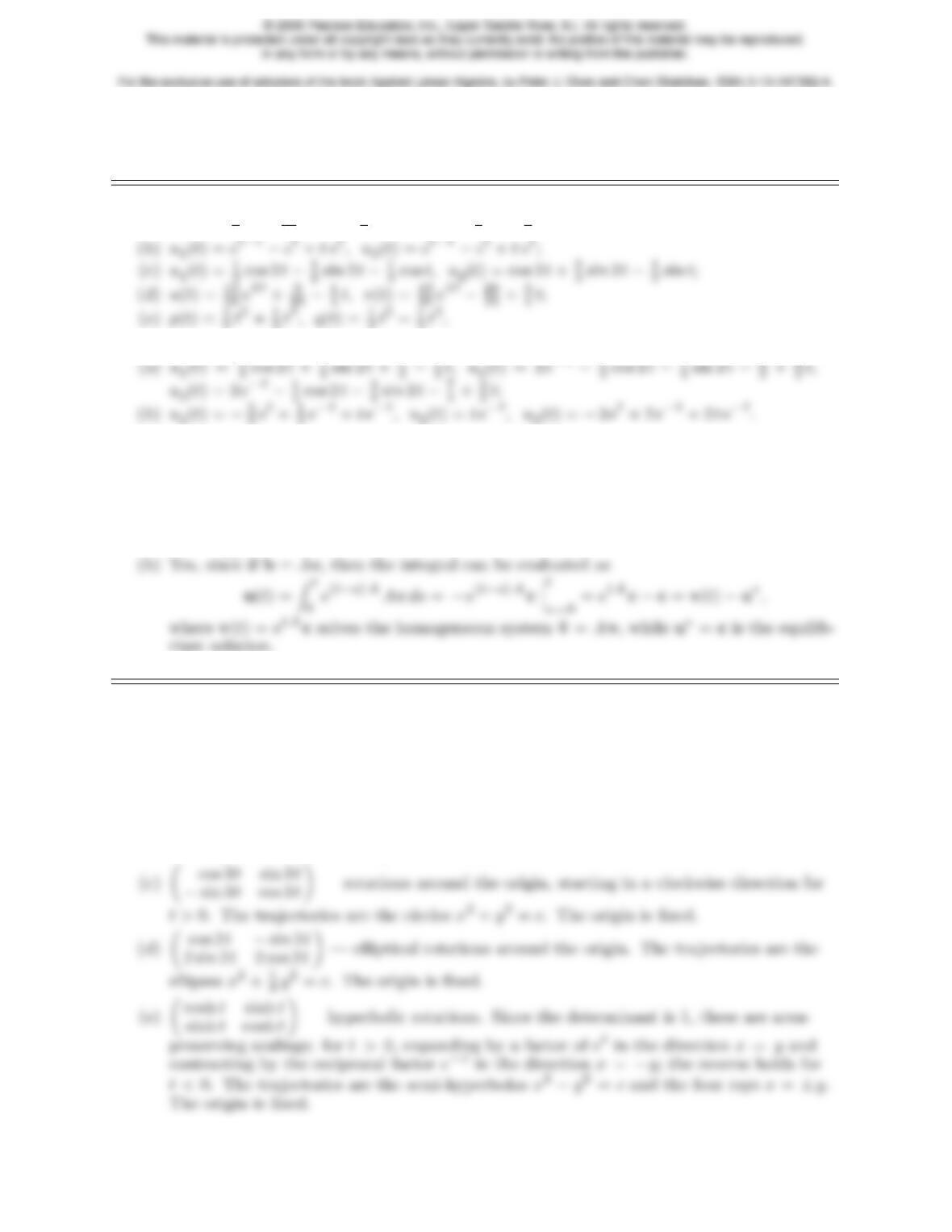
♥9.4.30. (a) All matrix exponentials are nonsingular by the remark after (9.44). (b) Both A=

256

9.4.31. Even though this formula is correct in the scalar case, it is false in general. Would that

life were so simple!

9.4.32.

(a)u1(t) = 1

3et−1

12 e−2t−1

4e2t, u2(t) = 1

3et−1

3e−2t;

9.4.33.

9.4.34. Since λis not an eigenvalue, A−λI is nonsingular. Set w= (A−λI )−1v. Then

u⋆(t) = eλ t wis a solution. The general solution is u(t) = eλ t w+z(t) = eλ t w+et Ab,

where bis any vector.

9.4.35.

(a)u(t) = Zt

0e(t−s)Abds.

9.4.36.

(a) e2t0

0 1 !— scalings in the xdirection, which expand when t > 0 and contract when

t < 0. The trajectories are half-lines parallel to the xaxis. Points on the yaxis are left

fixed.

(b) 1 0

t1!— shear transformations in the ydirection. The trajectories are lines parallel

to the yaxis. Points on the yaxis are fixed.

257