Mathematics Chapter 8 where Λ is the diagonal eigenvalue matrix

(c) Eigenvalues: 7,1; eigenvectors: 1

2

1!, 1

0!.

B

6

C

B

C

B

2

C

♦8.4.10. If L[v] = λv, then, using the inner product,

λkvk2=hL[v],vi=hv, L[v]i=λkvk2,

which proves that the eigenvalue λis real. Similarly, if L[w] = µw, then

λhv,wi=hL[v],wi=hv, L[w]i=µhv,wi,

and so if λ6=µ, then hv,wi= 0.

♦8.4.11. As shown in the text, since yi∈V⊥, its image Ayi∈V⊥also, and hence Ayiis a

(b) Using Exercise 8.2.13(c),

∆ωk= (S−I )ωk=“1−e2k π i/n ”ωk,

and so ωkis an eigenvector of ∆ with corresponding eigenvalue 1 −e2k π i/n.

(c) Since Sis an orthogonal matrix, ST=S−1, and so STωk=e−2k π i/n ωk. Therefore,

Kωk= (ST−I )(S−I )ωk= (2 I −S−ST)ωk

222

if k=1

2n(which requires that nbe even), the eigenvector ωn/2= ( 1,−1,1,−1, . . . )T

is real.

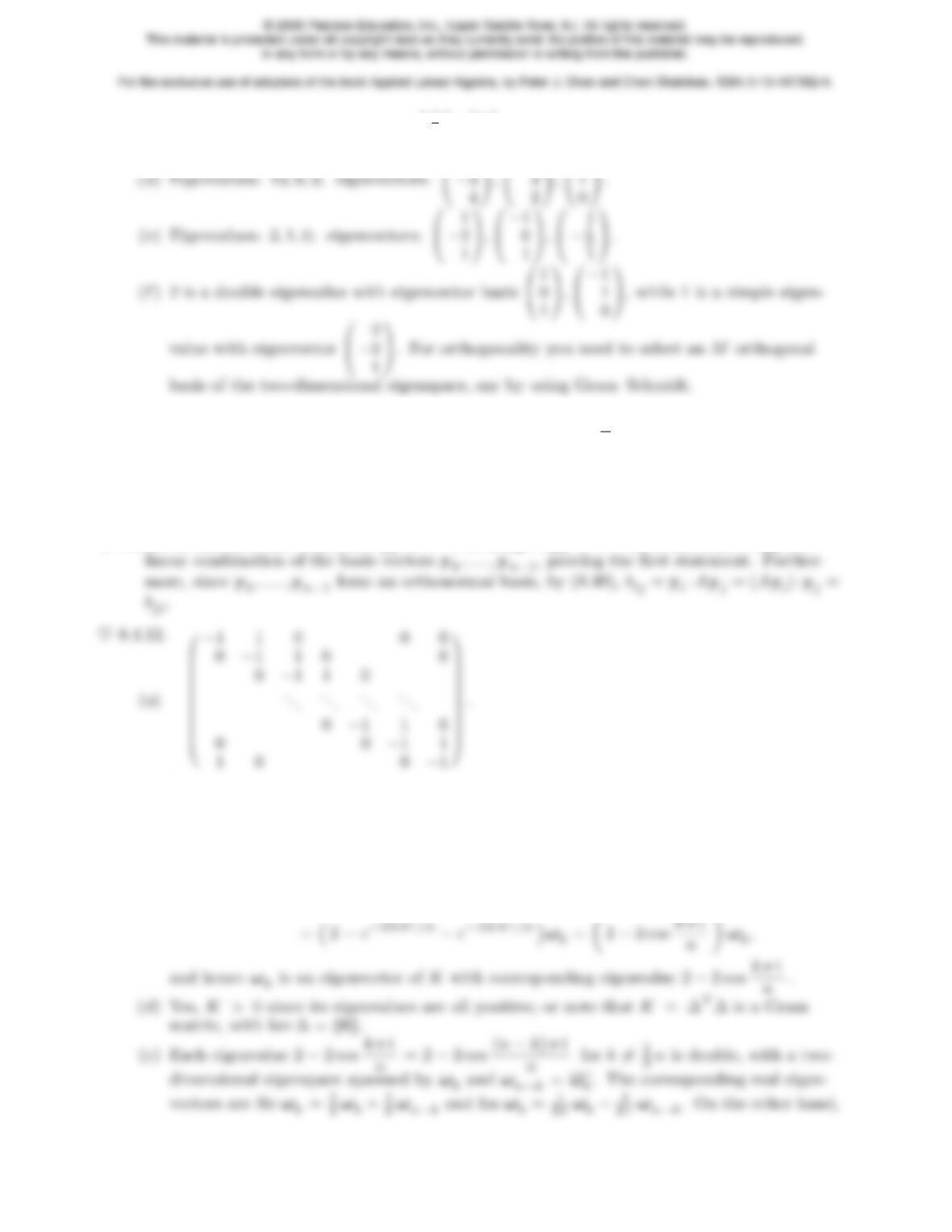
♥8.4.13.

(a) The shift matrix has c1= 1, ci= 0 for i6= 1; the difference matrix has c0=−1, c1= 1,

and ci= 0 for i > 1; the symmetric product Khas c0= 2, c1=cn−1=−1, and ci= 0

for 1 < i < n −2;

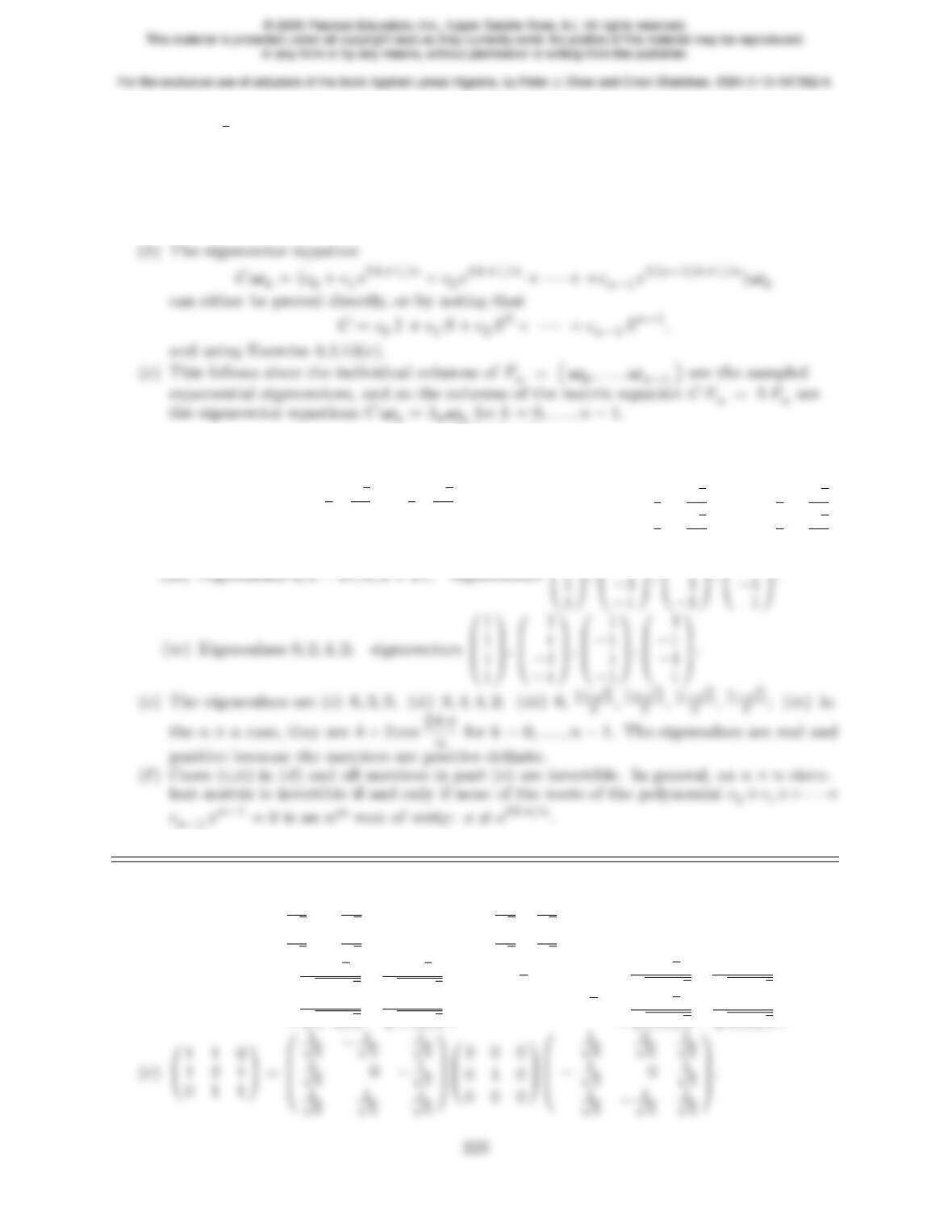
(d) (i) Eigenvalues 3,−1; eigenvectors 1

1!, 1

−1!.

(ii) Eigenvalues 6,−3

2−√3

2i,−3

2+√3

2i ; eigenvectors 0

B

@

1

11

C

A,0

B

@

1

−1

2+√3

2i

−1

2−√3

2i

1

C

A,0

B

@

1

−1

2−√3

2i

−1

2+√3

2i

1

C

A.

B

1

C

B

1

i

1

C

B

1

−1

1

C

B

1

−i

1

C

8.4.14.

(a) −3 4

4 3 !=0

B

@

1

√5−2

√5

2

√5

1

√5

1

C

A 5 0

0−5!0

B

@

1

√5

2

√5

−2

√5

1

√5

1

C

A.

(b) 2−1

−1 4 !=0

B

@

1−√2

√4−2√2

1+√2

√4+2√2

1

√4−2√2

1

√4+2√2

1

C

A 3 + √2 0

0 3 −√2!0

B

@

1−√2

√4−2√2

1

√4−2√2

1+√2

√4+2√2

1

√4+2√2

1

C

A.

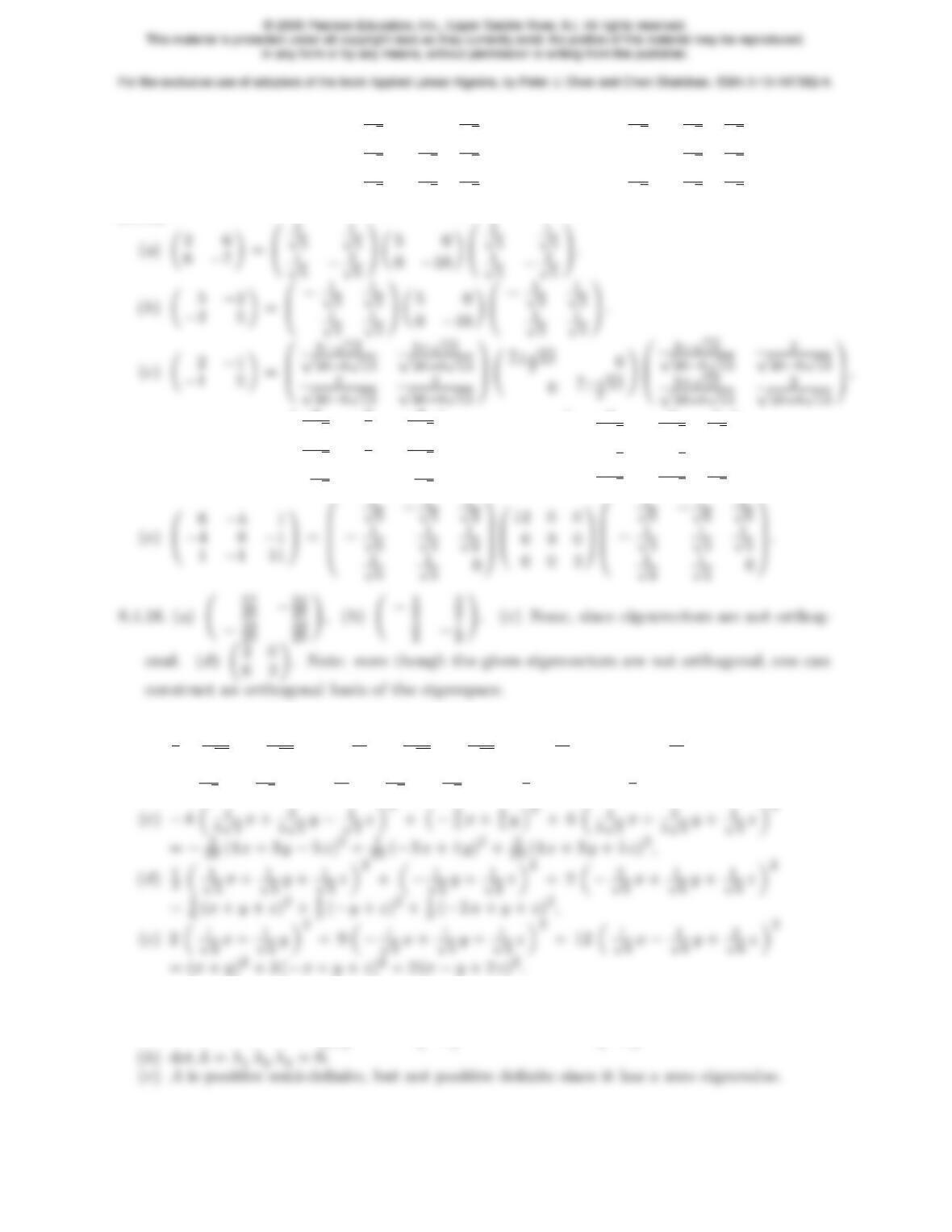
(d)0

B

@

3−1−1

−1 2 0

−1 0 2 1

C

A=0

B

@

−2

√601

√3

1

√6−1

√2

1

√3

1

√6

1

√2

1

√3

1

C

A0

B

@

4 0 0

020

0 0 1

1

C

A0

B

@

−2

√6

1

√6

1

√6

0−1

√2

1

√2

1

√3

1

√3

1

√3

1

C

A.

8.4.15.

(d)0

B

@

1 0 4

013

4 3 1 1

C

A=0

B

@

4

5√2−3

5−4

5√2

3

5√2

4

53

5√2

1

√201

√2

1

C

A0

B

@

6 0 0

0 1 0

0 0 −4

1

C

A0

B

@

4

5√2

3

5√2

1

√2

−3

54

50

−4

5√2−3

5√2

1

√2

1

C

A,

1

8.4.17.

(a)1

2„3

√10 x+1

√10 y«2+11

2„−1

√10 x+3

√10 y«2=1

20 (3x+y)2+11

20 (−x+ 3y)2,

(b) 7 „1

√5x+2

√5y«2+11

2„−2

√5x+1

√5y«2=7

5(x+ 2y)2+2

5(−2x+y)2,

♥8.4.18.

(a)λ1=λ2= 3,v1=0

B

@

1

01

C

A,v2=0

B

@−1

0

11

C

A,λ3= 0,v3=0

B

@

1

−1

11

C

A;

224

01

♦8.4.19. The simplest is A= I . More generally, any matrix of the form A=STΛS, where

S= ( u1u2… un) and Λ is any real diagonal matrix.

8.4.20. True, assuming that the eigenvector basis is real. If Qis the orthogonal matrix formed

by the eigenvector basis, then AQ =QΛ where Λ is the diagonal eigenvalue matrix. Thus,

A=QΛQ−1=QΛQT=ATis symmetric. For complex eigenvector bases, the result is

8.4.21. Using the spectral factorization, we have xTAx= (QTx)TΛ(QTx) =

n

X

i= 1

λiy2

i, where

yi=ui·x=kxkcos θidenotes the ith entry of QTx.

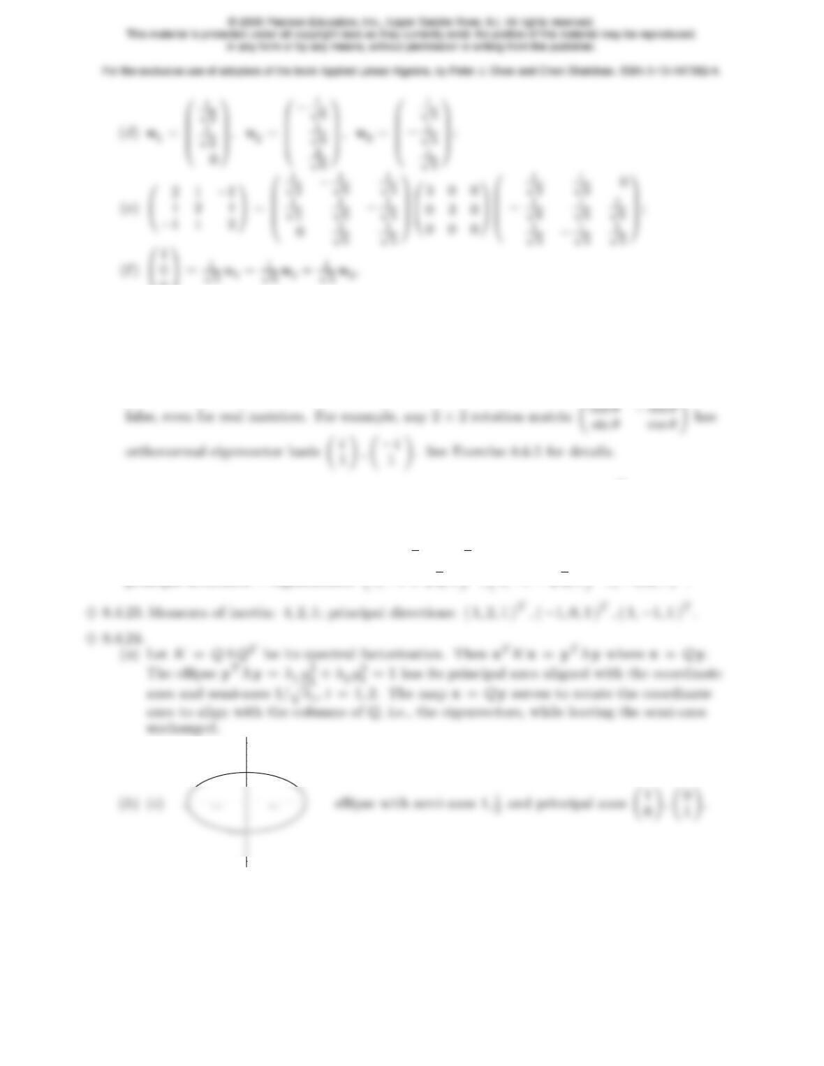
8.4.22. Principal stretches = eigenvalues: 4 + √3,4−√3,1;

principal directions = eigenvectors: “1,−1 + √3,1”T,“1,−1−√3,1”T,(−1,0,1 )T.

-1

0.5

1

225

(ii)

-1.5 -1 -0.5 0.5 1 1.5

-1.5

-1

-0.5

0.5

1

1.5

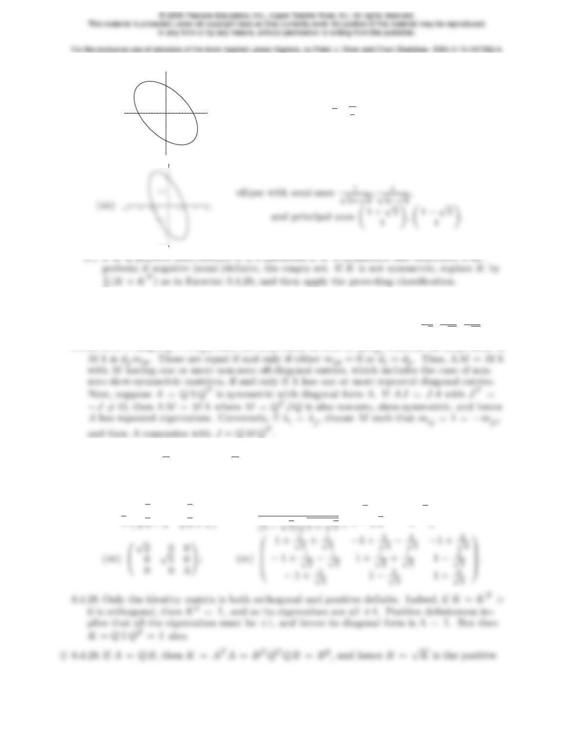
ellipse with semi-axes √2,q2

3, and principal axes −1

1!, 1

1!.

-1.5

1.5

2(K+KT) as in Exercise 3.4.20, and then apply the preceding classification.

♦8.4.25. (a) Same method as in Exercise 8.4.24. Its principal axes are the eigenvectors of K,

and the semi-axes are the reciprocals of the square roots of the eigenvalues. (b) Ellipsoid

with principal axes: ( 1,0,1 )T,(−1,−1,1 )T,(−1,2,1 )Tand semi-axes 1

√6,1

√12 ,1

√24 .

8.4.26. If Λ = diag (λ1, . . . , λn), then the (i, j) entry of Λ Mis dimij , whereas the (i, j) entry of

♦8.4.27.

(a) Set B=Q√ΛQT, where √Λ is the diagonal matrix with the square roots of the eigen-

values of Aalong the diagonal. Uniqueness follows from the fact that the eigenvectors

and eigenvalues are uniquely determined. (Permuting them does not change the final

form of B.)

(b) (i)1

√3−1√3 + 1 !; (ii )1

226

8.4.30. (a) 0 1

2 0 != 0 1

1 0 ! 2 0

0 1 !, (b) 2−3

1 6 !=0

B

@

1

√5

2

√5

C

A √5 0

0 3√5!,

(c) 1 2

0 1 !=0

B

@

1

√2

1

√2

−1

√2

1

√2

1

C

A0

B

@

1

√2

1

√2

1

√2

3

√2

1

C

A,

B

0−3 8

C

B

0−3

54

5

1

C

B

1 0 0

C

(ii) (a) −3 4

4 3 != 50

@

1

52

5

2

54

51

A−50

@

4

5−2

5

−2

51

A.

(b) 2−1

−1 4 != (3 + √2 )0

B

@

3−2√2

4−2√2

1−√2

4−2√2

1−√2

1

C

A+ (3 −√2 )0

B

@

3+2√2

4−2√2

1+√2

4−2√2

1+√2

1

C

A.

♦8.4.32. According to Exercise 8.4.7, the eigenvalues of an n×nHermitian matrix are all real,

and the eigenvectors corresponding to distinct eigenvalues orthogonal with respect to the

8.4.33.

(a) 3 2 i

−2 i 6 !=0

B

@

i

√5

2

√5

−2 i

√5

1

√5

1

C

A 2 0

0 7 !0

B

@−i

√5

2 i

√5

2

√5

1

√5

1

C

A,

227

8.4.34. Maximum: 7; minimum: 3.

8.4.36.

(a)5+√5

2= max{2x2−2xy + 3y2|x2+y2= 1 },

8.4.38. (a) Maximum: 3; minimum: −2; (b) maximum: 5

2; minimum: −1

2;

(c) maximum: 8+√5

2= 5.11803; minimum: 8−√5

2= 2.88197;

(d) maximum: 4+√10

2= 3.58114; minimum: 4−√10

2=.41886.

8.4.41. max{xTKx|kxk= 1 }=λ1is the largest eigenvalue of K. On the other hand, K−1

is positive definite, cf. Exercise 3.4.10, and hence min{xTK−1x|kxk= 1 }=µnis its

smallest eigenvalue. But the eigenvalues of K−1are the reciprocals of the eigenvalues of K,

and hence its smallest eigenvalue is µn= 1/λ1, and so the product is λ1µn= 1.

8.4.44. Note that vTKv

kvk2=uTKu, where u=v

kvkis a unit vector. Moreover, if vis orthogo-

nal to an eigenvector vi, so is u. Therefore, by Theorem 8.30

max 8

<

:

vTKv

kvk2˛˛˛˛˛˛v6=0,v·v1=··· =v·vj−1= 0 9

=

;

= max nuTKu˛˛˛kuk= 1,u·v1=··· =u·vj−1= 0 o=λj

.

♥8.4.45.

(a) Let R=√Mbe the positive definite square root of M, and set f

K=R−1K R−1. Then

xTKx=yTf

Ky,xTMx=yTy=kyk2, where y=Rx. Thus,

8.4.46. (a) Maximum: 3

4, minimum: 2

5; (b) maximum: 9+4√2

7, minimum: 9−4√2

7;

(c) maximum: 2, minimum: 1

2; (d) maximum: 4, minimum: 1.

8.5.1. (a) 3 ±√5, (b) 1, 1; (c) 5√2; (d) 3,2; (e)√7,√2; (f) 3,1.

8.5.2.

(a) 1 1

0 2 !=0

B

@

−1+√5

√10−2√5−1−√5

√10+2√5

2

√10−2√5

2

√10+2√5

1

C

A0

@q3 + √5 0

0q3−√51

A0

B

@

−2+√5

√10−4√5

1

√10−4√5

−2−√5

√10+4√5

1

√10+4√5

1

C

A,

229

8.5.3.

(a) 1 1

0 1 !=0

B

@

1+√5

√10+2√5

1−√5

√10−2√5

2

√10+2√5

2

√10−2√5

1

C

A0

@q3

2+1

2√5 0

0q3

2−1

2√51

A0

B

@

−1+√5

√10−2√5

2

√10−2√5

−1−√5

√10+2√5

2

√10+2√5

1

C

A;

(b) The first and last matrices are proper orthogonal, and so represent rotations, while the mid-

dle matrix is a stretch along the coordinate directions, in proportion to the singular values. Ma-

trix multiplication corresponds to composition of the corresponding linear transformations.

8.5.4.

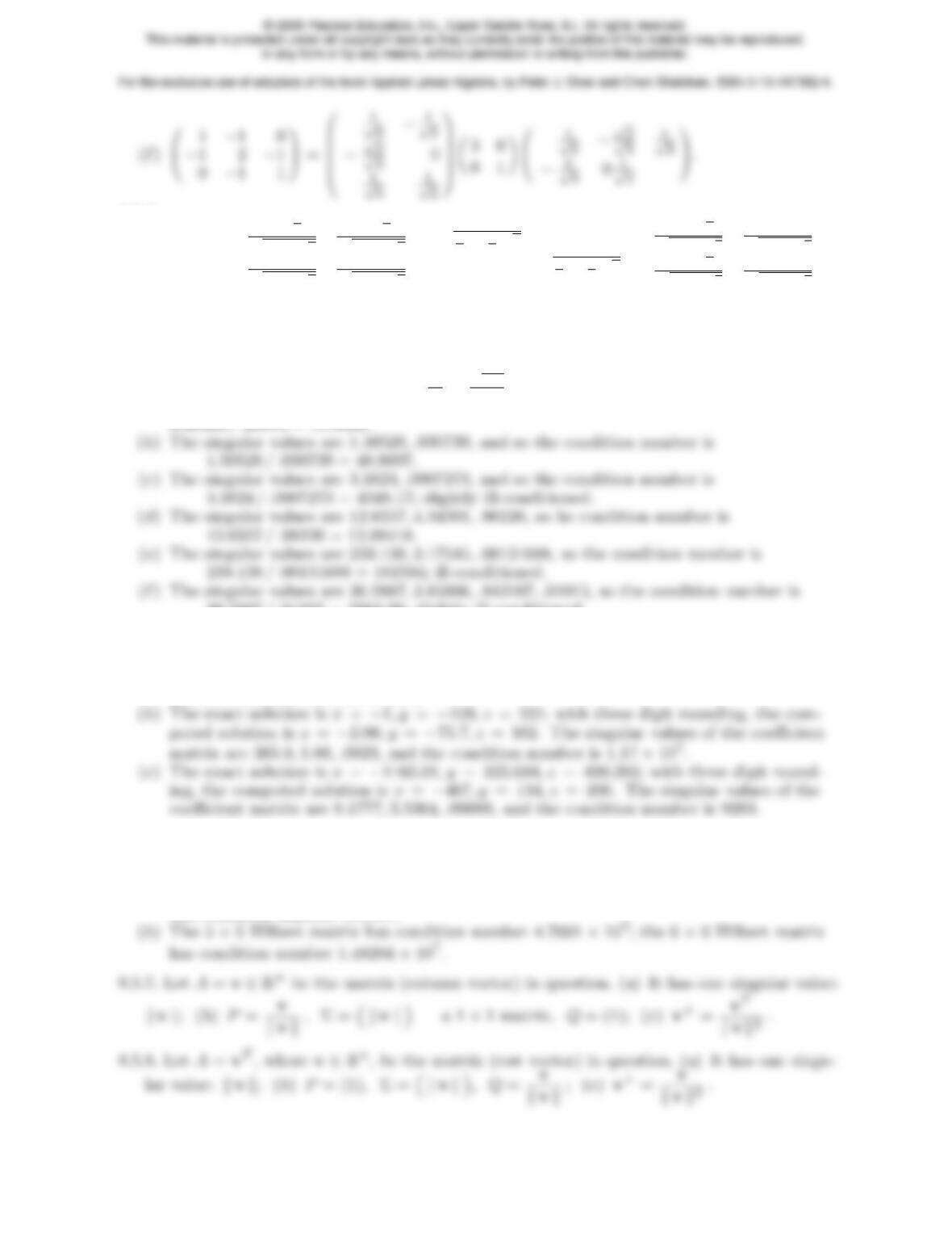
(a) The eigenvalues of K=ATAare 15

2±√221

2= 14.933, .0667. The square roots of these

eigenvalues give us the singular values of A. i.e., 3.8643, .2588. The condition number is

30.2887 / .01015 = 2984.09; slightly ill-conditioned.

♠8.5.5. In all cases, the large condition number results in an inaccurate solution.

(a) The exact solution is x= 1, y =−1; with three digit rounding, the computed solution is

x= 1.56, y =−1.56. The singular values of the coefficient matrix are 1615.22, .274885,

and the condition number is 5876.

♠8.5.6.

(a) The 2×2 Hilbert matrix has singular values 1.2676, .0657 and condition number 19.2815.

The 3 ×3 Hilbert matrix has singular values 1.4083, .1223, .0027 and condition number

524.057. The 4 ×4 Hilbert matrix has singular values 1.5002, .1691, .006738, .0000967

and condition number 15513.7.

230

8.5.9. Almost true, with but one exception — the zero matrix.

8.5.10. Since S2=K=ATA, the eigenvalues λof Kare the squares, λ=σ2of the eigenvalues

8.5.11. True. If A=PΣQTis the singular value decomposition of A, then the transposed

equation AT=QΣPTgives the singular value decomposition of AT, and so the diagonal

entries of Σ are also the singular values of AT.

♦8.5.13.

(a) When Ais nonsingular, all matrices in its singular value decomposition (8.40) are square.

Thus, we can compute det A= det Pdet Σ det QT=±1 det Σ = ±σ1σ2··· σn,since

the determinant of an orthogonal matrix is ±1. The result follows upon taking absolute

values of this equation and using the fact that the product of the singular values is non-

negative.

matrix with singular values 10kand 10−k, has condition number 102k.

8.5.14. False. For example, the diagonal matrix with entries 2 ·10kand 10−kfor k≫0 has

determinant 2 but condition number 2 ·102k.

8.5.15. False — the singular values are the absolute values of the nonzero eigenvalues.

8.5.18. False. This is only true if Sis an orthogonal matrix.

♥8.5.19.

(a) If kxk= 1, then y=Axsatisfies the equation yTBy= 1, where B=A−TA−1=

PTΣ−2P. Thus, by Exercise 8.4.24, the principal axes of the ellipse are the columns of

231

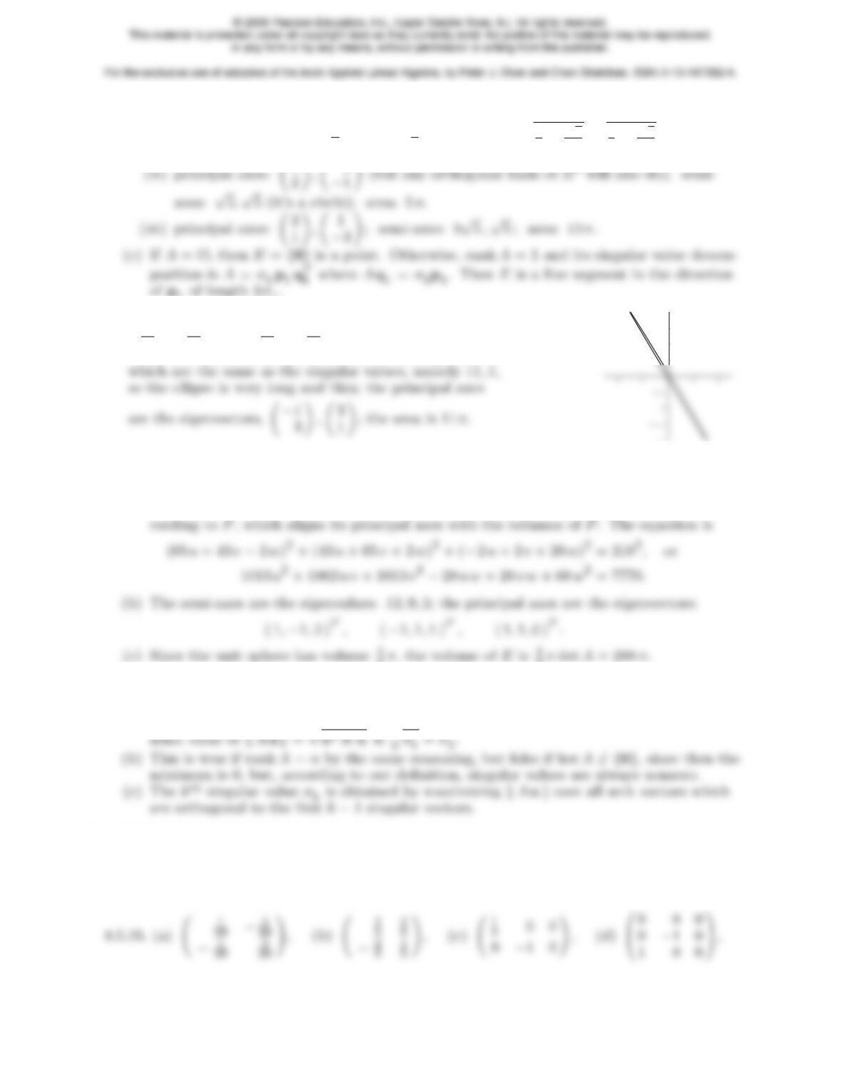
axes. Thus, area E=π σ1σ2=π|det A|using Exercise 8.5.13.

(d) (i) principal axes: 2

1 + √5!, 2

1−√5!; semi-axes: r3

2+√5

2,r3

2−√5

2; area: π.

8.5.20.

“10

11 u+3

11 v”2+“3

11 u+2

11 v”2= 1 or 109u2+ 72uv + 13v2= 121.

Since Ais symmetric, the semi-axes are the eigenvalues,

-10

2.5

5

7.5

10

8.5.21.

(a) In view of the singular value decomposition of A=PΣQT, the set Eis obtained by

first rotating the unit sphere according to QT, which doesn’t change it, then stretching

it along the coordinate axes into an ellipsoid according to Σ, and then rotating it ac-

3π, the volume of Eis 4

3πdet A= 288 π.

♦8.5.22.

(a)kAuk2= (Au)TAu=uTKu, where K=ATA. According to Theorem 8.28,

max{uTKu| kuk= 1 }is the largest eigenvalue λ1of K=ATA, hence the maxi-

♦8.5.23. Let λ1be the maximal eigenvalue, and let u1be a corresponding unit eigenvector. By

Exercise 8.5.22, σ1≥ kAu1k=|λ1|.

8.5.24. By Exercise 8.5.22, the numerator is the largest singular value, while the denominator is

the smallest, and so the ratio is the condition number.

232

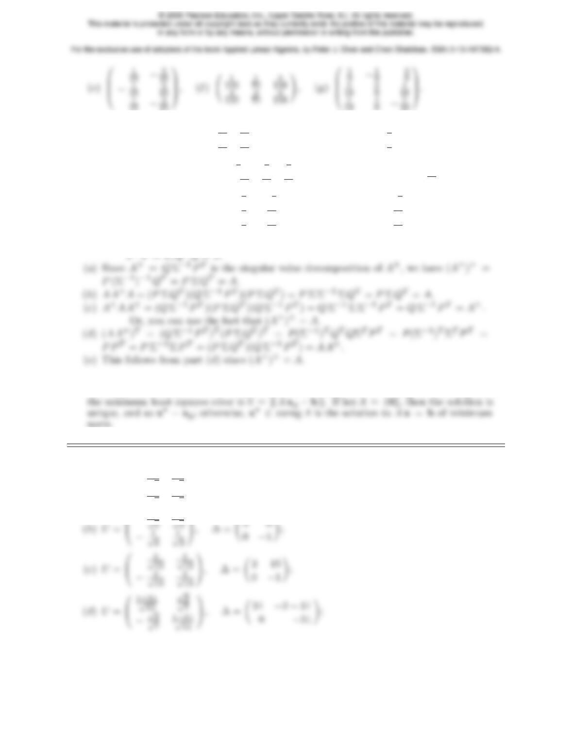
8.5.26.

(a)A= 1 1

3 3 !, A+=0

@

1

20 3

20

1

20 3

20 1

A,x⋆=A+ 1

−2!=0

@−1

4

−1

41

A;

(b)A=0

B

@

1−3

2 1

1 1 1

C

A, A+=0

@

1

61

31

6

−3

11 1

A,x⋆=A+0

B

@

2

−1

01

C

A= 0

−7

11 !;

(c)A= 1 1 1

2−1 1 !, A+=0

B

@

1

72

7

4

7−5

14

2

71

14

1

C

A,x⋆=A+ 5

2!=0

B

@

9

7

15

7

11

7

1

C

A.

♥8.5.27. We repeatedly use the fact that the columns of P, Q are orthonormal, and so

8.5.28. In general, we know that x⋆=A+bis the vector of minimum norm that minimizes the

least squares error kAx−bk. In particular, if b∈rng A, so b=Ax0for some x0, then

8.6.1.

(a)U=0

B

@

1

√2

1

√2

−1

√2

1

√2

1

C

A,∆ = 2−2

0 2 !;

1

√2

1

√2

1

233

8.6.2. If Uis real, then U†=UTis the same as its transpose, and so (8.45) reduces to UTU=

I , which is the condition that Ube an orthogonal matrix.

♦8.6.3. If U†

1U1= I = U†

2U2, then (U1U2)†(U1U2) = U†

2U†

1U1U2=U†

2U2= I , and so U1U2is

also orthogonal.

♦8.6.4. If Ais symmetric, its eigenvalues are real, and hence its Schur Decomposition is A=

k=i|aik |2,and hence aik = 0 for all k > i. Therefore Ais a diagonal matrix.

(e) Let U= ( u1u2. . . un) be the corresponding unitary matrix, with U−1=U†. Then

AU =UΛ, where Λ is the diagonal eigenvalue matrix, and so A=UΛU†=UΛU†.

Then AA†=UΛU†UΛ†U†=UΛΛ†U†=A†Asince ΛΛ†= Λ†Λ as it is diagonal.

(f) Let A=U∆U†be its Schur Decomposition. Then, as in part (e), AA†=U∆∆†U†,

while A†A=U∆†∆U†. Thus, Ais normal if and only if ∆ is; but part (d) says this

happens if and only if ∆ = Λ is diagonal, and hence A=UΛU†satisfies the conditions

of part (e).

(g) If and only if it is symmetric. Indeed, by the argument in part (f), A=QΛQTwhere Q

is real, orthogonal, which is just the spectral factorization of A=AT.

8.6.6.

(a) One 2 ×2 Jordan block; eigenvalue 2; eigenvector e1.

234

8.6.7.

0

B

@

2 0 0 0

0 2 0 0

0 0 2 0

0 0 0 2

1

C

A,0

B

@

2 1 0 0

0 2 0 0

0 0 2 0

0 0 0 2

1

C

A,0

B

@

2 0 0 0

0 2 1 0

0 0 2 0

0 0 0 2

1

C

A,0

B

@

2 0 0 0

0 2 0 0

0 0 2 1

0 0 0 2

1

C

A,

8.6.9.

(a) Eigenvalue: 2. Jordan basis: v1= 1

0!,v2= 0

1

3!. Jordan canonical form: 2 1

0 2 !.

(b) Eigenvalue: −3. Jordan basis: v1= 1

2!,v2= 1

2

0!.

(e) Eigenvalues: −2,0. Jordan basis: v1=0

B

@−1

0

11

C

A,v2=0

B

@

−1

01

C

A,v3=0

B

@

−1

11

C

A.

Jordan canonical form: 0

B

@−2 1 0

0−2 0

0 0 0 1

C

A.

B

−2

1

C

B

1

0

1

C

B

−1

2

1

C

B

0

1

C

This material is protected under all copyright laws as they currently exist. No portion of this material may be reproduced,

in any form or by any means, without permission in writing from the publisher.

For the exclusive use of adopters of the book Applied Linear Algebra, by Peter J. Olver and Cheri Shakiban. ISBN 0-13-147382-4.

8.6.11. True. All Jordan chains have length one, and so consist only of eigenvectors.

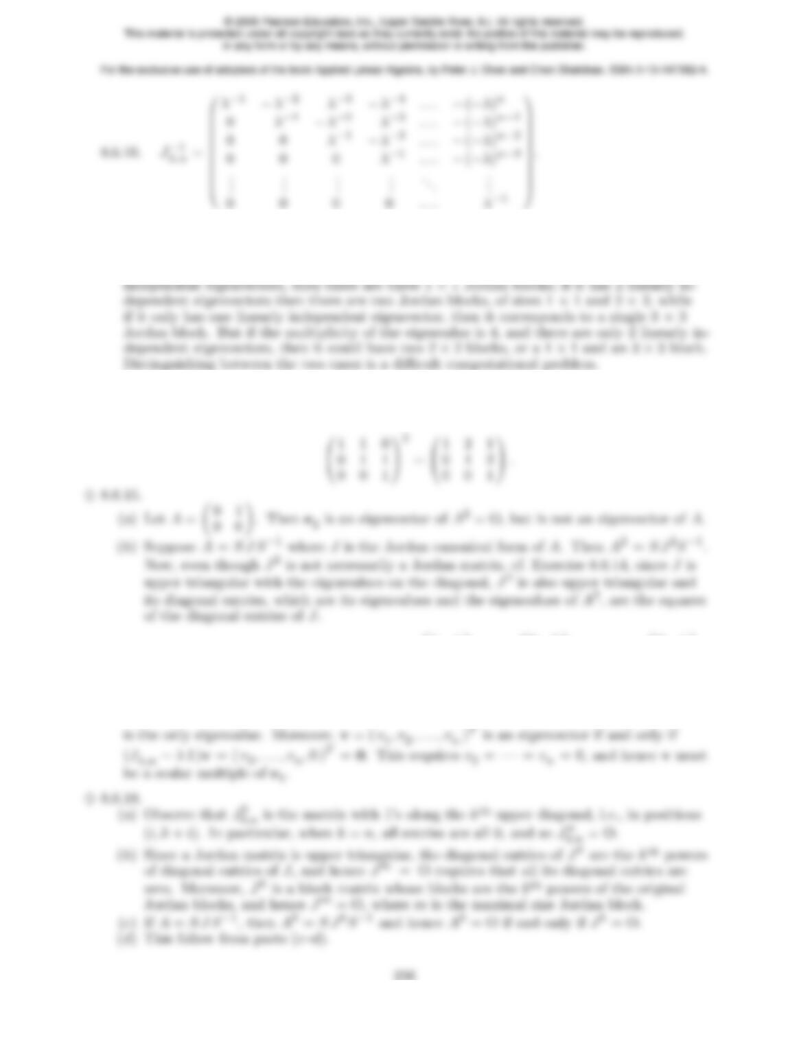
♦8.6.12. No in general. If an eigenvalue has multiplicity ≤3, then you can tell the size of its Jor-

dan blocks by the number of linearly independent eigenvectors it has: if it has 3 linearly

8.6.13. True. If zj=cwj, then Azj=cAwj=c λwj+cwj−1=λzj+zj−1.

8.6.14. False. Indeed, the square of a Jordan matrix is not necessarily a Jordan matrix, e.g.,

8.6.16. Not necessarily. A simple example is A= 1 1

0 0 !,B= 0 1

0 0 !, so AB = 0 1

0 0 !,

whereas B A = 0 0

0 0 !.

♦8.6.17. First, since Jλ,n is upper triangular, its eigenvalues are its diagonal entries, and hence λ

8.6.19. (a) Since Jkis upper triangular, Exercise 8.3.12 says it is complete if and only if it is

a diagonal matrix, which is the case if and only if Jis diagonal, or Jk= O. (b) Write

A=S J S−1in Jordan canonical form. Then Ak=S JkS−1is complete if and only if Jkis

complete, so either Jis diagonal, whence Ais complete, or Jk= O and so Ak= O.

♥8.6.20.

(a) If D= diag (d1,…,dn), then pD(λ) =

n

Y

i=1

(λ−di). Now D−diI is a diagonal matrix

with 0 in its ith diagonal position. The entries of the product pD(D) =

n

Y

i=1

(D−diI ) of

diagonal matrices is the product of the individual diagonal entries, but each such prod-

(d) The determinant of a (Jordan) block matrix is the product of the determinants of the

individual blocks. Moreover, by part (c), substituting Jinto the product of the charac-

teristic polynomials for its Jordan blocks gives zero in each block, and so the product

matrix vanishes.

♦8.6.21. The nvectors are divided into non-null Jordan chains, say w1,k, . . . , wik,k, satisfying

Bwi,k =λkwi,k +wi−1,k with λk6= 0 the eigenvalue, (and w0,k =0by convention)

along with the null Jordan chains, say y1,l,…,wil,l,wil+1,l, supplemented by one addi-

tional vector, satisfying Byi,k =yi−1,k, and, in addition, the null vectors

z1, . . . , zn−r−k∈ker B\rng B. Suppose some linear combination vanishes:

237