Chapter 8
8.1
1
111
, …, 1 …
rn
aaa
nnn
111
8.2
12
Yxx
(a)
12 1 2
12
12
1212
12
11
() ( ) ( ) ( )
ii
EY E x x E x E x
nn
nn
nn
μμμμ
(b)
22
22
12
121122
2222
12
1212
1111
var( ) var( ) var( )
ii
Yx xnn
nn
nnnn
σσ
σσ
8.4
[1 ( 1)]
t
x
Me
θ
/
[1 ( 1)]
tn n
x
Me
θ
/
1/ / 1/
[1 ( 1)] [1 ( 1)]
tn n tn tn n tn
Mn e e e e
n
θ
θθθ
/
Chapter 8 113
μ
8.6
[1 ( 1)]
tn
x
Me
θ
μ
θ
(1 )
n
θθ
σ
[ / (1 )] / (1 )
/
()/
11
n
nt tn
xx
t
MeMe e
θθ θθ
μσ
μσ
θ
σ
Use series expansion to show that as n
2
(1/2)
()/
t
x
Me
μσ
8.7 (1) independent
(2) information bounded with
1
k
8.8 (1) independent
(2) uniformly bounded k = 2
114 Mathematical Statistics, 8E
2
2
2
2
11 1 1 11 1
1
23 4 49
11 1 1 1 1
1
22 2 4 4
11 1
1
24 4
n
Y
nnn
nn
n
n
σ
8.10
() 0
i
Ex
2
2
1
2
4
i
σ
2
11 1 1 1 1
var( ) 1
n
Yn nn
Chapter 8 115
8.11 When we sample with replacement from a finite population we satisfy all the conditions for
random sampling from an infinite population. The random variables
12
, , ,
n
xx x
are
independent and identically distributed.
8.12 Hypergeometric distribution applies to sampling without replacement from a finite population
k
N
μ
Consider population of k 1′s and
Nk
0’s.
8.15 (a)
123 ( 1) 1
22
NNN N
NN
μ
1
2
x
N
μ
(b)
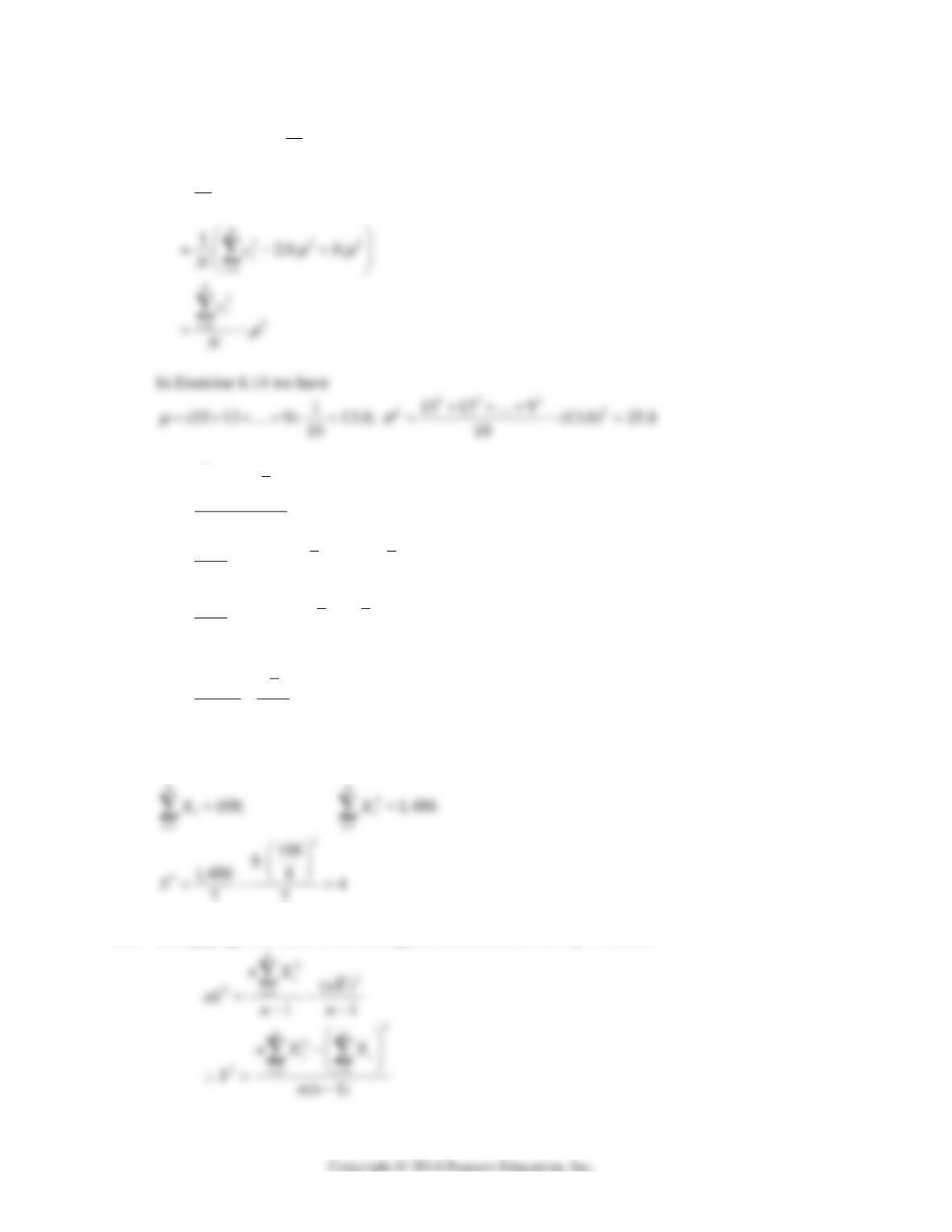
22 2 2 2 2
2
1 2 ( 1) ( 1)(2 1) ( 1) 1
46412
NN N N N N
N
σ
116 Mathematical Statistics, 8E
8.17
22
1
1
()
N
i
i
cN
σμ
22
11
12
NN
ii
ii
ccN
N
μ
μ
8.18
2
21
()
1
n
i
i
XX
Sn
22
11
222
1
2
2
1
12)
1
12
1
11
nn
ii
ii
n
i
i
n
i
i
XXXnX
n
XnXnX
n
XnX
nn
From the given data we calculate
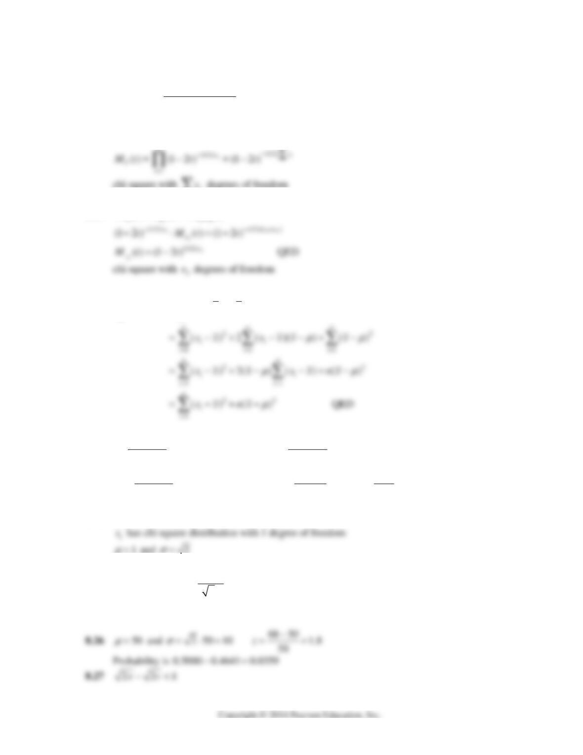
8.19 Multiplying both sides of the last equation in Exercise 8.18 by n we have
Chapter 8 117
Substituting the data of Exercise 8.18 we obtain
2
2
8(1, 486) (108) 4
8(7)
S
8.20
(1/2)
() (1 2)
i
i
v
x
Mt t
i
Yx
i
8.21
() () ()
xx xx
MtMt M t
8.22
2
2
11
() ()()
nn
ii
ii
xxxx
μ
μ
8.23
2
2
(1) 1
nS
En
σ
2
22
(1)
() 1
n
ES n
σσ
2
2
(1)
var 2( 1)
nS n
σ
44
2
2
2
var( ) 2( 1) 1
(1)
Sn
n
n
σσ
8.24 Follows directly from central limit theorem
8.25 From 8.24 with
(0,1)
2
n
Yn
zN
n
Here
n
Y
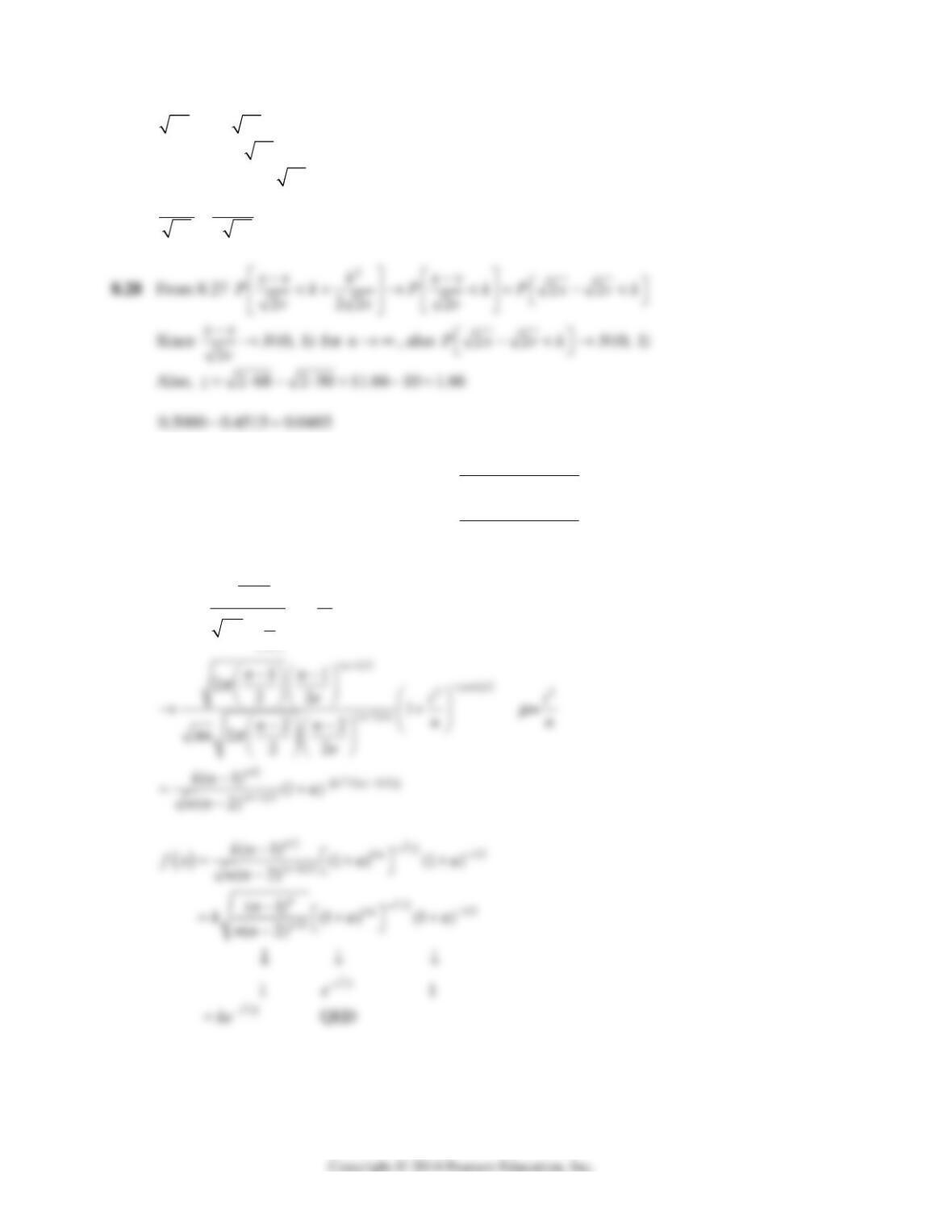
is a Chi-Square random variable with n degrees of freedom.
118 Mathematical Statistics, 8E
22xk v
2
2222xk k v v
2
22 22xvk kv
2
222
xv k k
vv
8.29 From 8.26 probability is 0.0359; % error = 0.0359 0.04596 100 21.9%
0.04596
From 8.27 probability is 0.0485; % error = 0.0485 0.04596 100 5.53%
0.04596
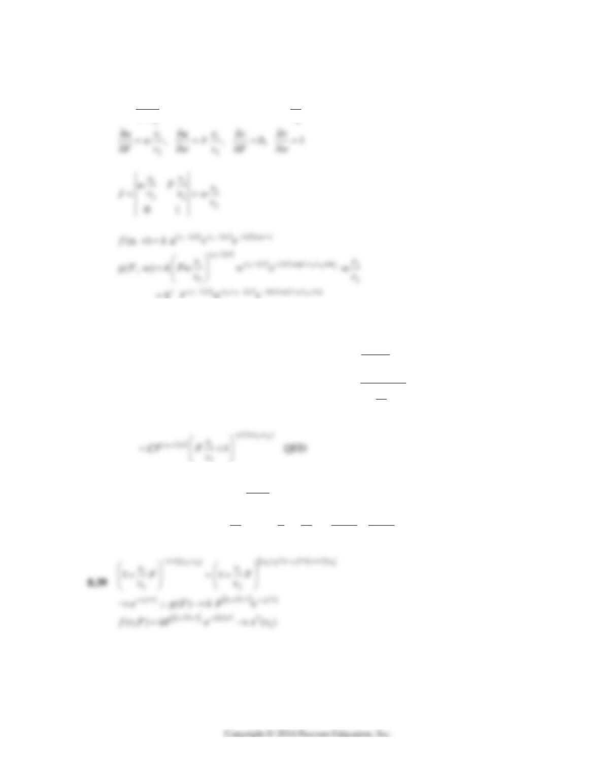
8.35
(1)/2
2
1
2
() 1
2
n
n
t
fx nn
n
π
Γ
Γ
Chapter 8 119
8.36 The Cauchy distribution
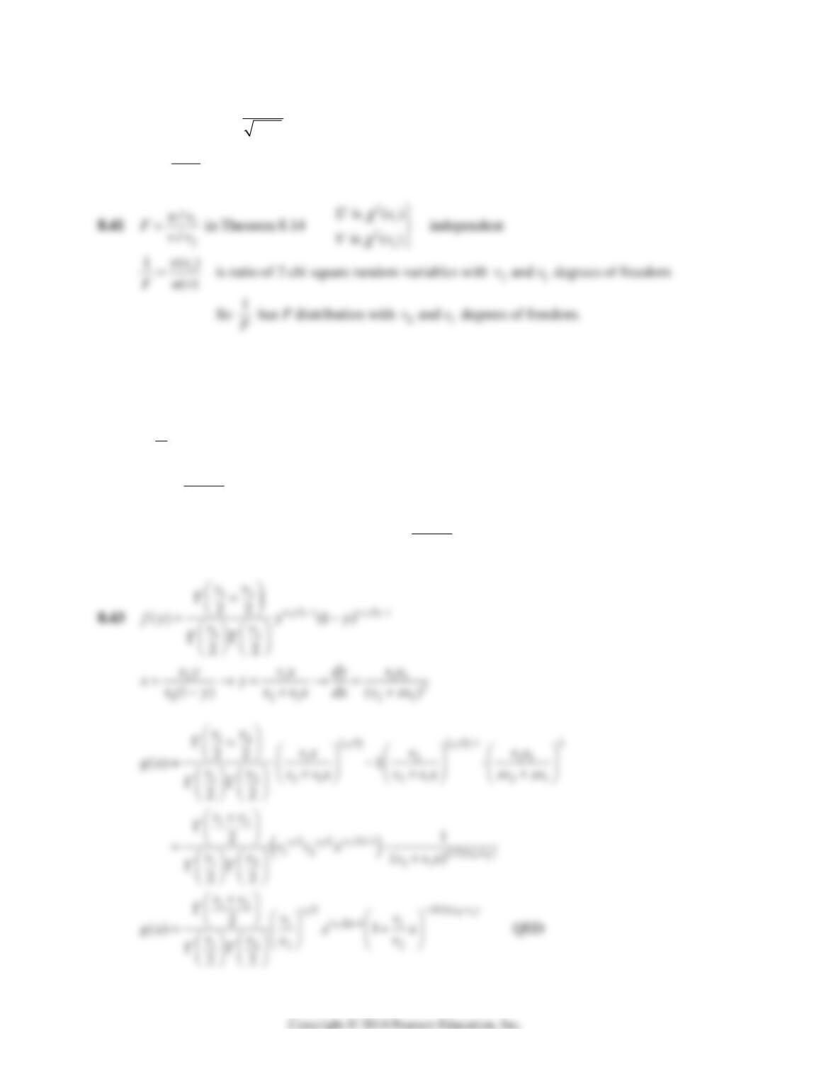
8.37 F =
1
/
/
uv
vv
wv
1
v
uFw
v
vw
kF w e
12 12
1
()/21(1/2)(/)1
(2)/2
0
()
vv Fvv
v
hF k F w e dw
Gamma distribution with
12
2
vv
α
1
2
2
1
v
Fv
β
2
8.38 Make use of the fact that
1
2
/
/
uv
Fvv
where u and v are independent chi square random
variables, so that
22 2
1
1122
11
( ) ( ) QED
22
vv v
EF EuE v
vvvvv
120 Mathematical Statistics, 8E
8.40 T defined as
/
Z
TYv
in Theorem 8.12 where Z + Y are independent.
2
2
/
Z
TYv
where
22
(1)Z
χ
by Theorem 8.7
2
()Yv
χ
QED
/
/
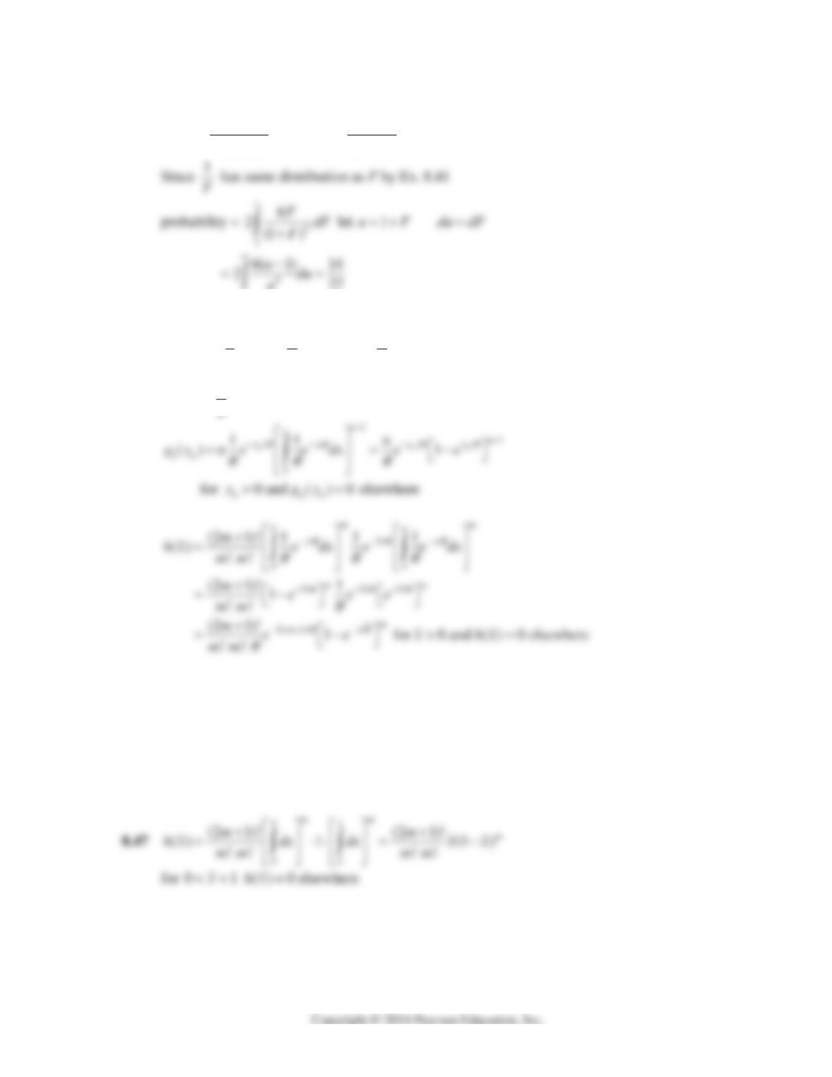
8.42
12
12
(, )
( , ) by Exercise 8.41
xFvv
yFvv
12
,,
()
vv
Px F
α
α
12
,,
1
()
vv
PF
Y
α
α
12
,,
1
vv
PY F
α
α
21
1,,vv
PY F
α
α
21
12
1,,
,,
1
vv
vv
FF
α
α
Chapter 8 121
8.44 Substituting into formula of Theorem 8.14 yields
4
4
(4) 6
() (1 )
(2) (2) (1 )
F
gF F F F
Γ
ΓΓ
3
u
8.45
111
1
1
1
1
////
11
/
111
11
() 8
for 0 and ( ) 0 elsewhere
n
n
yyyx
y
yn
n
gy ne e dx e e
neygy
θθθθ
θ
θθ
θ
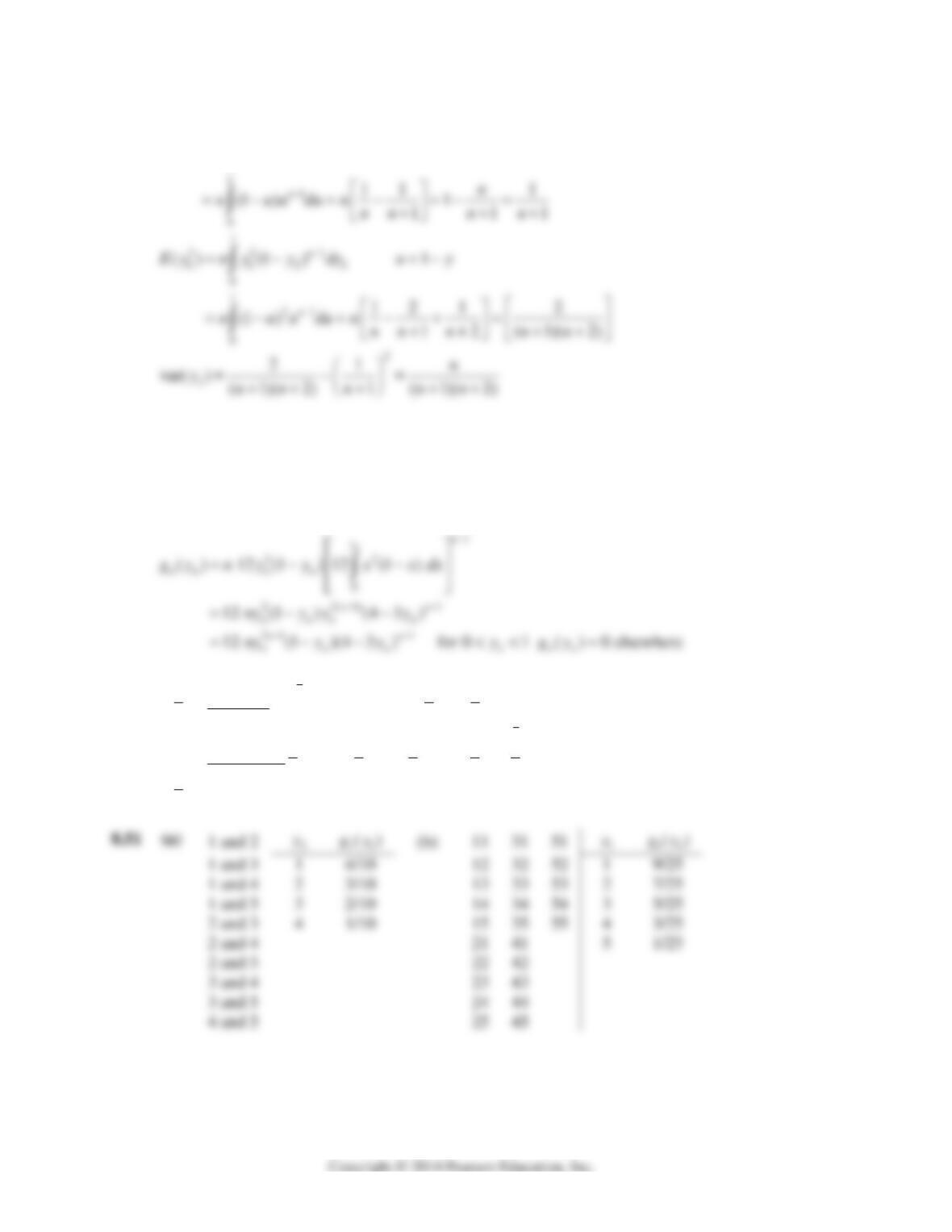
8.46
1
1
1
1
11 1 1 11
( ) 1 (1 ) for 0 1 ( ) 0 elsewhere
n
n
y
gy n dx n y y gy
1
1
0
( ) 1 for 0 1 ( ) 0 elsewhere
n
n
y
n
nn n n nn
gy n dx ny y gy
122 Mathematical Statistics, 8E
8.48
1
1
1111 1
0
( ) (1 ) let 1
n
Ey n y y dy u y
8.49
1
1
1
22
11 1 1
1
234
11 11 1 11
() 12 (1 )12 (1 )
12 (1 ) 1 4 3 for 0 1 ( ) 0 elsewhere
n
y
n
gy n y y x xdx
ny y y y y g y
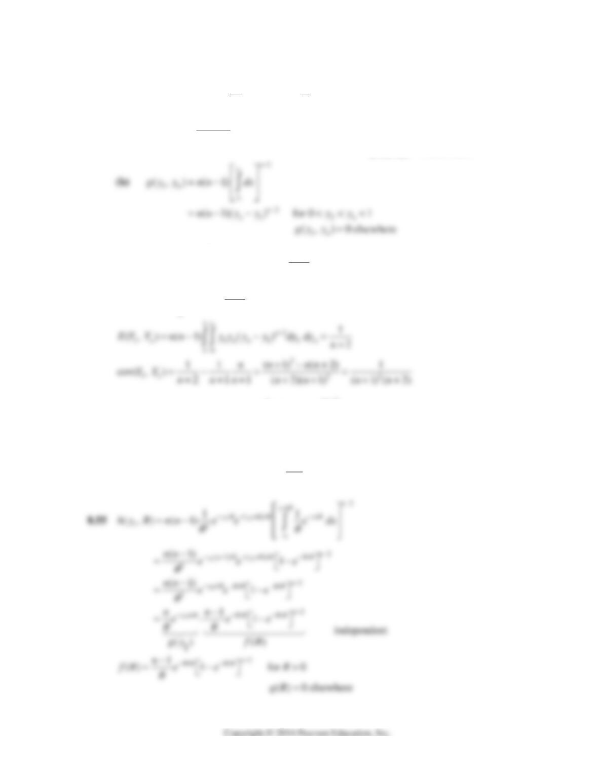
8.50
1
222
0
32 3 4
(2 1)!
() 12 (1 ) 12 (1 )12 (1 )
! !
12(2 1)! (1 )[4 3 ] [1 4 3 ]
! !
mm
x
x
mmm
m
h x x x dx x x x x dx
mm
mxxxxx
mm
( ) 0 elsewherehx
Chapter 8 123
8.52 (a)
1
11
2
/
//
12
2
(1/ )( ) //
1
2
11
(, ) ( 1)
(1) for 0
n
n
nn
n
y
y
yx
n
y
n
yy yy
n
gy y nn e e e dx
nn eee yy
θ
θθ
θθθ
θ
θ
θ
1
( , ) 0 elsewhere
n
gy y
8.53 From 8.48
1
1
1111
0
1
() (1 ) 1
n
Ey n y y dy n
and
1
0
() 1
n
nnn
n
EY n y dy n
8.54
1
1
2
111
(, ) ( 1)()( ) ()
n
yR
y
hy R nn f y f y R f x dx
Let
1n
yyR
and transform holding
1
y
fixed.
1
n
dR
dy
124 Mathematical Statistics, 8E
8.56
1
1
2
2
1
(, ) ( 1) ( 1)
n
yR
n
y
hy R nn dx nn R
1
011Ry
and 0 elsewhere
8.58 (a)
1
()
n
y
y
pfxdx
()
n
n
dp fy
dy
22
11 2
1
1
(, ) ( 1)()( ) ( 1)( )
()
nn
n
hy p nn f y f y p nn f y p
fy
8.59 Density of P is same density as R obtained in Exercise 8.56, so the formula for the mean and
the variance are the same as those obtained in Exercise 8.57. When n is large
( ) 1 and var( ) 0Ep p
.
Chapter 8 125
8.61 (a)
11
12 495
4
(b)
1 120 1
22 12 21 20 77
5
8.63 (a) It is divided by 2
120 / 30 2
(b) It is divided by 1.5
180 / 80 1.5
(c) It is multiplied by 3
450 / 50 3
(d) It is multiplied by 2.5
250 / 40 2.5
8.64 (a)
200 5 0.9799;
200 1
(b)
300 50 0.8361;
300 1
(c)
800 200 0.7509
800 1
8.66
6.3 0.7
9
x
σ
129.4 128 2
0.7
(a) Probability is at most
1
126 Mathematical Statistics, 8E
8.70
6.8 0.85
8
x
σ
(a)
52.9 51.4 1.765
0.85
z
0.5 0.4612 0.0388
8.71
25 2.5
100
x
σ
31.2
2.5
z
1 2(0.3849) 1 0.7698 0.2302
8.74
12
78 75 3
xx
μ
12
150 200 3
30 50
xx
σ
4.8 3 0.6
3
z
0.5 0.2257 0.2743
Chapter 8 127
8.76
2
1
1 1 0.9375 0.0625, 4k
k
(0.4)(0.6) (0.25)(0.75) 0.00048 0.00047 0.0308
500 400
σ
It will fail between
0.40 0.25 0.15 4(0.0308) 0.15 0.1232k
σ
0.0268 and 0.2732
8.78 n = 16
2
25
σ
2
2
15 0.6
25
s
ys
has chi-square distribution with 15 degrees of freedom
probability
0.6(54.668) ( 32.801) 0.005yPy
probability
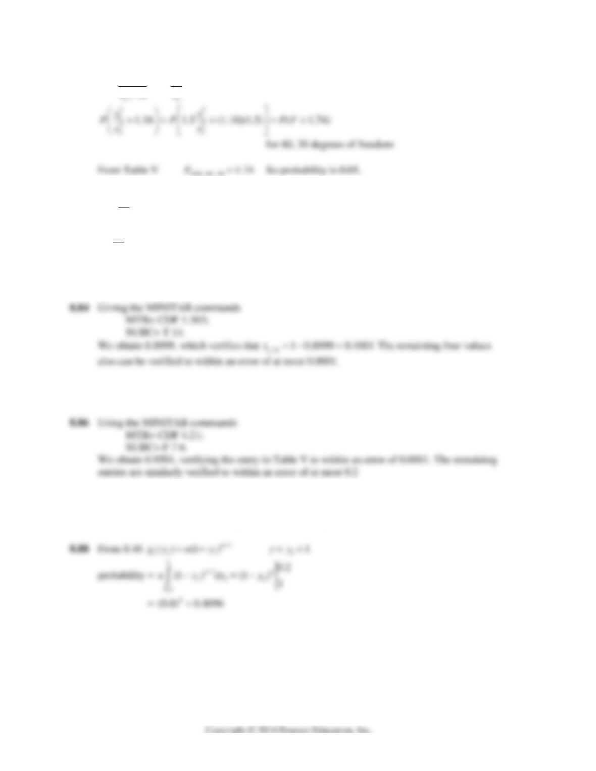
0.6(12.102) ( 7.2612) 0.05yPy
total probability = 0.055
8.79
2
4
σ
9n
2
2
82
4
s
ys
128 Mathematical Statistics, 8E
8.82
22
11
22
/12 1.5
ss
Fss
0.05, 60, 30
8.83
2
1
2
2
s
Fs
2
1
2
2
4.03 1 ( 4.03)
s
PPF
s
with 9 and 14 degrees of freedom
From Table VI
0.01, 9, 14
4.03F
So probability =
10.01 0.99
8.85 Following the procedure of Exercise 8.84, but using 21 in place of 11, we verify all five table
entries to four decimal places.
8.87 Following the procedure of Exercise 8.86, but using
SUBC> F 12 17
We obtain 0.9900. The remaining entries are similarly verified
Chapter 8 129
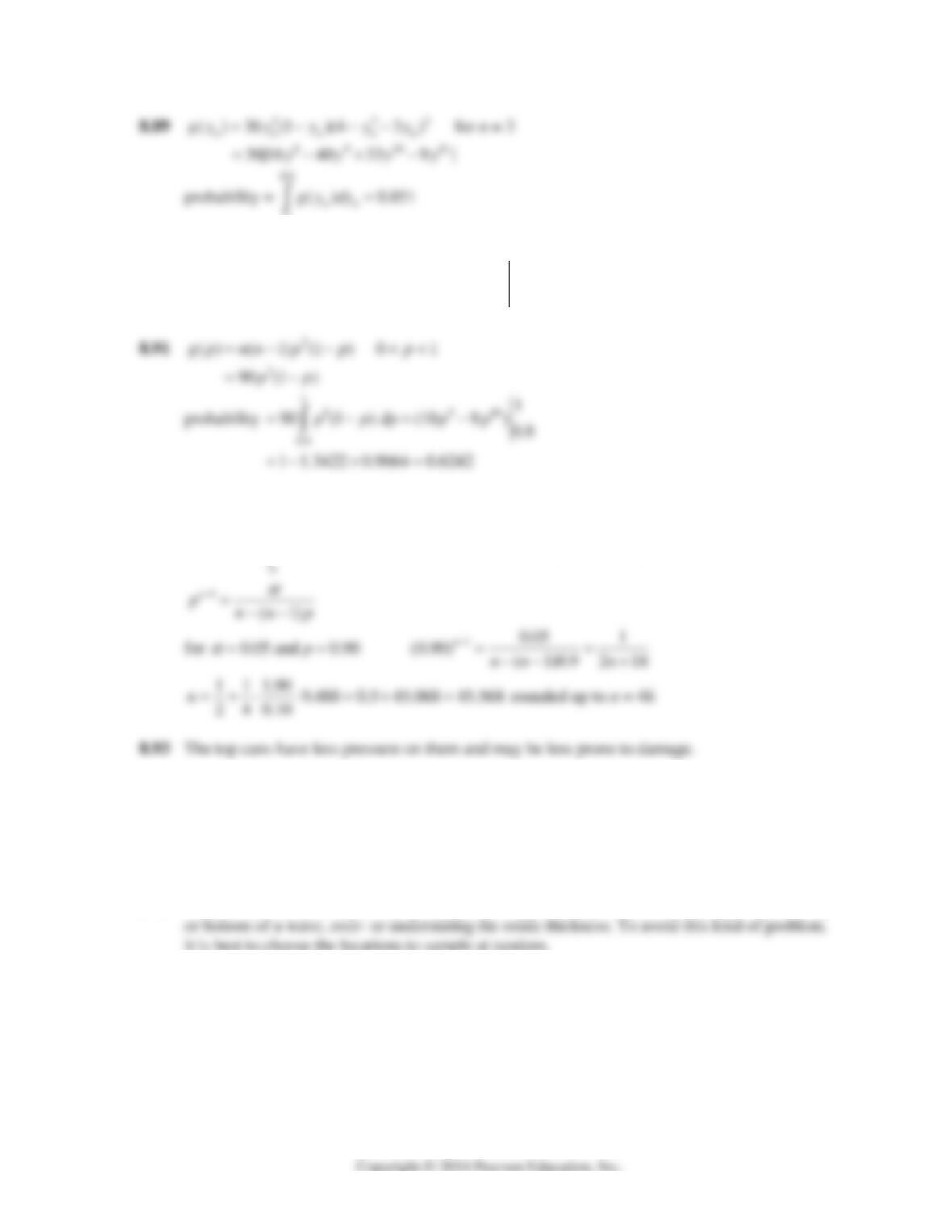
0
8.90
2
( ) 20 (1 ) for 0 1gR R R R
probability =
1
34 4 5
0.75
1
20 ( ) (5 4 ) 0.3672
0.75
RRdR R R
8.92
2
() ( 1) (1 )
n
gp nn p p
21 1
(1) (1 ) (1) (1)
p
nnnn
n n p p dp np n p p n n p
α
8.94 (a) The sample, without the “bad” parts, will make the lathe seem better than it is.
(b) The sample is representative of product produced by the lather after inspection.
8.95 The sample is more likely to include longer sections than shorter ones; they take more time to
pass the inspection station.
8.96 A systematic sample (e.g. every so many millimeters) may produce results always near the top