Mathematics Chapter 8 The equilibrium solution is asymptotically stable

Solutions — Chapter 8

8.1.1. (a)u(t) = −3e5t, (b)u(t) = 3e2(t−1), (c)u(t) = e−3(t+1).

8.1.2. γ= log 2/100 ≈.0069. After 10 years: 93.3033 gram; after 100 years: 50 gram;

after 1000 years: .0977 gram.

8.1.6. The solution is u(t) = u(0) e.27 t. For the given initial conditions, u(t) = 1,000,000 when

t= log(1000000/5000)/.27 = 19.6234 years.

8.1.8. (a)u(t) = 1

2+1

2e2t, (b)u(t) = −3, (c)u(t) = 2 −3e−3(t−2).

8.1.9. (a)du

dt =−log 2

1000 u+ 5 ≈ −.000693 u+ 5. (b) Stabilizes at the equilibrium solution

u⋆= 5000/log 2 ≈721 tons. (c) The solution is u(t) = 5000

♦8.1.11. (a)|u1(t)−u2(t)|=ea t |u1(0) −u2(0) | → ∞ when a > 0, since u1(0) = u2(0) if and

only if the solutions are the same. (b)t= log(1000/.05)/.02 = 495.17.

8.1.12.

(a)u(t) = 1

3e2t/7.

206

This material is protected under all copyright laws as they currently exist. No portion of this material may be reproduced,

in any form or by any means, without permission in writing from the publisher.

For the exclusive use of adopters of the book Applied Linear Algebra, by Peter J. Olver and Cheri Shakiban. ISBN 0-13-147382-4.

♦8.1.13. According to Exercise 3.6.24, du

dt =caea t =au, and so u(t) is a valid solution. By

Euler’s formula (3.84), if Re a > 0, then u(t)→ ∞ as t→ ∞, and the origin is an unstable

equilibrium. If Re a= 0, then u(t) remains bounded t→ ∞, and the origin is a stable

equilibrium. If Re a < 0, then u(t)→0 as t→ ∞, and the origin is an asymptotically

stable equilibrium.

8.2.1.

(a) Eigenvalues: 3,−1; eigenvectors: −1

1!, 1

1!.

(f) Eigenvalues: 1,√6,−√6; eigenvectors: 0

B

@

2

0

11

C

A,0

B

@

−1 + √3

√2

2 + √3

√2

C

A

,0

B

@

−1−√3

√2

2−√3

√2

C

A

.

(i)−1 is a simple eigenvalue, with eigenvector 0

B

@

2

−1

11

C

A;

2 is a double eigenvalue, with eigenvectors 0

B

@

1

3

0

C

A,0

B

@

−2

3

1

C

A.

207

8.2.2. (a) The eigenvalues are e±iθ= cos θ±i sin θwith eigenvectors 1

∓i!. They are real

only for θ= 0 and π. (b) Because Rθ−aI has an inverse if and only if ais not an eigen-

value.

8.2.3. The eigenvalues are ±1 with eigenvectors ( sin θ, ±1−cos θ)T.

8.2.4. (a) O, and (b)−I , are trivial examples.

0 1 0

8.2.7.

(a) Eigenvalues: i ,−1 + i ; eigenvectors: 1

0!, −1

1!.

(b) Eigenvalues: ±√5; eigenvectors: i (2 ±√5)

8.2.8.

(a) Since Ov=0= 0v, we conclude that 0 is the only eigenvalue; all nonzero vectors v6=0

are eigenvectors.

8.2.9. For n= 2,the eigenvalues are 0,2, and the eigenvectors are −1

1!, and 1

1!.For n= 3,

−1

1

208

♦8.2.10.

(a) If Av=λv, then A(cv) = cAv=c λ v=λ(cv) and so cvsatisfies the eigenvector

equation for the eigenvalue λ. Moreover, since v6=0, also cv6=0for c6= 0, and so cvis

a bona fide eigenvector.

8.2.11. True — by the same computation as in Exercise 8.2.10(a), cvis an eigenvector for the

same (real) eigenvalue λ.

♦8.2.12. Write w=x+ i y. Then, since λis real, the real and imaginary parts of the eigenvector

equation Aw=λware Ax=λx, A y=λy, and hence x,yare real eigenvectors of A.

Thus x=a1v1+···+akvk,y=b1v1+···+bkvkfor a1, . . . , ak, b1, . . . , bk∈R, and hence

w=c1v1+··· +ckvkwhere cj=aj+ i bj.

8.2.14. (a) Eigenvalues: −3,1,5; eigenvectors: ( 2,−3,1 )T,“−2

3,−1,1”T,( 2,1,1 )T;

(b) tr A= 3 = −3 + 1 + 5, (c) det A=−15 = (−3) ·1·5.

8.2.15.

(a) tr A= 2 = 3 + (−1); det A=−3 = 3 ·(−1).

(b) tr A=5

6=1

2+1

3; det A=1

6=1

2·1

3.

8.2.16.

(a)a=a11 +a22 +a33 = tr A,b=a11 a22 −a12 a21 +a11 a33 −a13 a31 +a22 a33 −a23 a32,

8.2.17. If Uis upper triangular, so is U−λI , and hence p(λ) = det(U−λI ) is the product of

the diagonal entries, so p(λ) = Q(uii −λ). Thus, the roots of the characteristic equation

are u11, . . . , unn — the diagonal entries of U.

♦8.2.18. Since Ja−λI is an upper triangular matrix with λ−aon the diagonal, its determinant

is det(Ja−λI ) = (a−λ)nand hence its only eigenvalue is λ=a, of multiplicity n. (Or use

Exercise 8.2.17.) Moreover, (Ja−aI )v= ( v2, v3,…,vn,0 )T=0if and only if v=ce1.

8.2.21. (a) False. For example, 0 is an eigenvalue of both 0 1

0 0 !and 0 0

1 0 !, but the eigen-

8.2.22. False in general, but true if the eigenvectors coincide: If Av=λvand Bv=µv, then

AB v= (λµ)v, and so vis an eigenvector with eigenvalue λ µ.

♦8.2.23. If AB v=λv, then B Aw=λw, where w=Bv. Thus, as long as w6=0, it is

an eigenvector of B A with eigenvalue λ. However, if w=0, then AB v=0, and so the

8.2.26. Recall that Ais singular if and only if ker A6={0}. Any v∈ker Asatisfies Av=0=

0v. Thus ker Ais nonzero if and only if Ahas a null eigenvector.

8.2.27. Let v,wbe any two linearly independent vectors. Then Av=λvand Aw=µwfor

8.2.28. If λis a simple real eigenvalue, then there are two real unit eigenvectors: uand −u.

For a complex eigenvalue, if uis a unit complex eigenvector, so is eiθu, and so there are

210

8.2.29. All false. Simple 2 ×2 examples suﬃce to disprove them:

Strt with 0−1

1 0 !, which has eigenvalues i ,−i ; (a) 0−1

1−2!has eigenvalue −1;

(b) 1 0

0−1!has eigenvalues 1,−1; (c) 0−4

1 0 !has eigenvalues 2 i ,−2 i .

8.2.31.

(a) (i)Q= −1 0

0 1 !. Eigenvalues −1,1; eigenvectors 1

0!, 0

1!. (ii )Q=0

@

7

25 −24

25

−24

25 −7

25 1

A.

3

4

1 0 0

♦8.2.32.

(a)det(B−λI ) = det(S−1AS −λI ) = dethS−1(A−λI )Si

= det S−1det(A−λI ) det S= det(A−λI ).

(b) The eigenvalues are the roots of the common characteristic equation.

(c) Not usually. If wis an eigenvector of B, then v=Swis an eigenvector of Aand con-

versely.

8.2.33.

(a)pA−1(λ) = det(A−1−λI ) = det “λ A−1 1

λI−A!#=(−λ)n

det ApA 1

λ!.

Or, equivalently, if

pA(λ) = (−1)nλn+cn−1λn−1+··· +c1λ+c0,

211

♥8.2.34.

(a) If Av=λvthen 0=Akv=λkvand hence λk= 0, so λ= 0.

(b)A= 0 1

0 0 !has A2= 0 0

0 0 !;

A=0

B

@

011

0 0 1

0 0 0 1

C

Ahas A2=0

B

@

0 0 1

0 0 0

0001

C

A,A3=0

B

@

0 0 0

000

0 0 0 1

C

A.

In general, Acan be any upper triangular matrix with all zero entries on the diagonal,

and all nonzero entries on the super-diagonal.

♥8.2.35.

(a) det(AT−λI ) = det(A−λI )T= det(A−λI ), and hence Aand AThave the same

characteristic polynomial, which implies that they have the same eigenvalues.

8.2.36.

(a) The characteristic equation of a 3 ×3 matrix is a real cubic polynomial, and hence has at

least one real root. (b)0

B

@

0 1 0 0

−1 0 0 0

0 0 0 1

0 0 −1 0

1

C

A

has eigenvalues ±i . (c) No, since the characteris-

212

8.2.38. If Pv=λvthen P2v=λ2v. Since Pv=P2v, we find λv=λ2v. Since v6=0, it

follows that λ2=λ, so the only eigenvalues are λ= 0,1. All v∈rng Pare eigenvectors

8.2.39. False. For example, 0

B

@

100

0 1 0 1

C

Ahas eigenvalues 1, −1

2±√3

2i .

8.2.40.

(a) According to Exercise 1.2.29, if z= ( 1,1, . . . , 1 )T, then Azis the vector of row sums of

8.2.41.

(a) If Qv=λv, then QTv=Q−1v=λ−1vand so λ−1is an eigenvalue of QT. Further-

more, Exercise 8.2.35 says that a matrix and its transpose have the same eigenvalues.

(b) If Qv=λv, then, by Exercise 5.3.16, kvk=kQvk=|λ| kvk, and hence |λ|= 1.

Note that this proof also applies to complex eigenvalues/eigenvectors, with k·k denoting

♦8.2.42.

(a) According to Exercise 8.2.36, a 3 ×3 orthogonal matrix has at least one real eigenvalue,

which by Exercise 8.2.41 must be ±1. If the other two eigenvalues are complex conju-

gate, µ±iν, then the product of the eigenvalues is ±(µ2+ν2). Since this must equal the

♦8.2.43.

(a) The axis of the rotation is the eigenvector vcorresponding to the eigenvalue +1. Since

Qv=v, the rotation fixes the axis, and hence must rotate around it. Choose an or-

thonormal basis u1,u2,u3, where u1is a unit eigenvector in the direction of the axis of

8.2.44. In general, besides the trivial invariant subspaces {0}and R3, the axis of rotation and

213

8.2.45.

(a) (Q−I )T(Q−I ) = QTQ−Q−QT+ I = 2 I −Q−QT=Kand hence Kis a Gram

matrix, which is positive semi-definite by Theorem 3.28.

(b) The Gram matrix is positive definite if and only if ker(Q−I ) = {0}, which means that

Qdoes not have an eigenvalue of 1.

♥8.2.47.

(a)M2= 0 1

1 0 !: eigenvalues 1,−1; eigenvectors 1

1!, −1

1!;

M3=0

B

@

0 1 0

1 0 1

0 1 0 1

C

A: eigenvalues −√2,0,√2; eigenvectors 0

B

@

1

−√2

11

C

A,0

B

@

−1

0

11

C

A,0

B

@

1

√2

11

C

A.

♥8.2.49. For k= 1,…,n,

λk= 2 cos 2k π

n,vk= cos 2k π

n,cos 4k π

n,cos 6k π

n, . . . , cos 2(n−1)k π

n,1!T

.

8.2.50. Note first that if Av=λv, then D v

0!= Av

0!=λ v

0!, and so v

0!is an eigen-

vector for Dwith eigenvalue λ. Similarly, each eigenvalue µand eigenvector wof Bgives

an eigenvector 0

w!of D. Finally, to check that Dhas no other eigenvalue, we compute

♥8.2.52.

214

(a)Bv= (A−v bT)v=Av−(b·v)v= (λ−β)v.

(b)B(w+cv) = (A−v bT)(w+cv) = µw+ (c(λ−β)−b·w)v=µ(w+cv) provided

c=b·w/(λ−β−µ).

(d) (i) The eigenvalues of Aare 6,2 and the eigenvectors 1

1!, −3

1!. The deflated ma-

trix B=A−λ1v1vT

1

kv1k2= 0 0

−2 2 !has eigenvalues 0,2 and eigenvectors 1

1!, 0

1!.

8.3.1. (a) Complete; dim = 1 with basis ( 1,1 )T. (b) Not complete; dim = 1 with basis

8.3.2.

(a) Eigenvalue: 2; eigenvector: 2

1!; not complete.

(b) Eigenvalues: 2,−2; eigenvectors: 2

1!, 1

1!; complete.

215

8.3.3.

(a) Eigenvalues: −2,4; the eigenvectors −1

1!, 1

1!form a basis for R2.

(b) Eigenvalues: 1 −3 i , 1 + 3 i ; the eigenvectors i

1!, −i

1!,are not real, so the dimen-

sion is 0.

(c) Eigenvalue: 1; there is only one eigenvector v1= 1

0!spanning a one-dimensional sub-

space of R2.

1

(h) The eigenvalues are −1,1,−i−1,−i + 1. The eigenvectors are 0

B

@

1

0

C

A

,0

B

@

3

2

6

C

A

,0

B

@

i

−i

1

C

A

,

0

B

@

−1

−i

i

1

C

A

. The real eigenvectors span a two-dimensional subspace of R4.

8.3.4. Cases (a,b,d,f,g,h) have eigenvector bases of Cn.

8.3.5. Examples: (a)0

B

@

1 1 0

0 1 1

0 0 1 1

C

A, (b)0

B

@

1 0 0

0 1 1

0 0 1 1

C

A.

216

8.3.8. (a) Every eigenvector of Ais an eigenvector of A2with eigenvalue λ2, and hence if A

has a basis of eigenvectors, so does A2. (b)A= 0 1

0 0 !with A2= O.

♦8.3.9. Suppose Av=λv. Write v=

n

X

i= 1

civi. Then Av=

n

X

i= 1

ciλiviand hence, by linear

independence, λici=λ ci. Thus, either λ=λior ci= 0.

8.3.10. (a) If Av=λv, then, by induction, Anv=λnv, and hence vis an eigenvector with

eigenvalue λn. (b) Conversely, if Ais complete and Anhas eigenvalue µ, then at least one

√µis an eigenvalue of A. Indeed, the eigenvector basis of A

8.3.13. Let V= ker(A−λI ). If v∈V, then Av∈Vsince (A−λI )Av=A(A−λI )v=0.

♦8.3.14.

(a) Let v=x+ i y,w=v=x−iybe the corresponding eigenvectors, so x=1

2v+1

2w,

y=−1

2iv+1

2iw. Thus, if cx+dy=0where c, d are real scalars, then

“1

2c−1

2id”v+“1

2c+1

2id”w=0.

Since v,ware eigenvectors corresponding to distinct eigenvalues µ+ i ν6=µ−iν,

Lemma 8.13 implies they are linearly independent, and hence

8.3.15. In all cases, A=SΛS−1.

(a)S= 3 3

1 2 !, Λ = 0 0

0−3!.

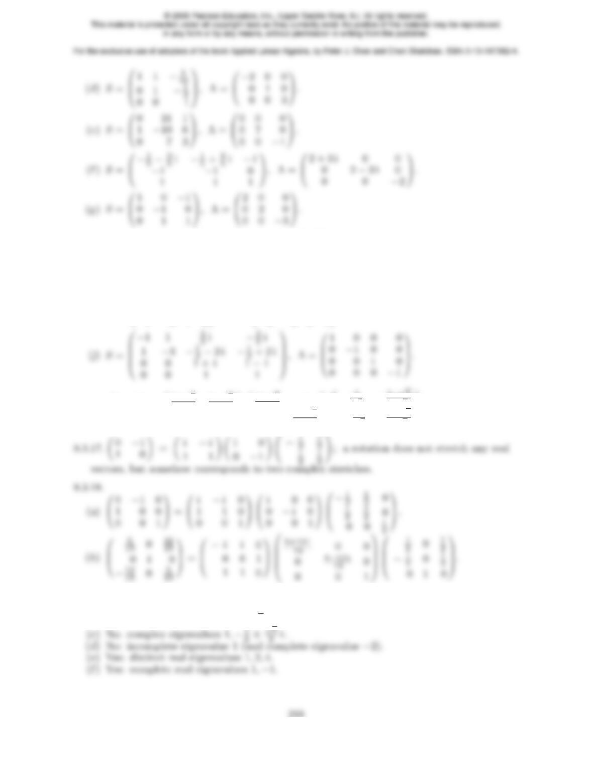
(h)S=0

B

@

−4 3 1 0

−3 2 0 1

0 6 0 0

12 0 0 0

1

C

A

, Λ = 0

B

@

−2 0 0 0

0−100

0 0 1 0

0 0 0 2

1

C

A

.

(i)S=0

B

@

0−1 0 1

−1 0 1 0

0 1 0 1

1 0 1 0

1

C

A

, Λ = 0

B

@

−1 0 0 0

0−1 0 0

0 0 1 0

0 0 0 1

1

C

A

.

8.3.16. 1 1

1 0 !=0

@

1+√5

21−√5

2

1 1 1

A0

@

1+√5

20

01−√5

2

1

A0

B

@

1

√5−1−√5

2√5

−1

√5

1+√5

2√5

C

A.

8.3.19.

(a) Yes: distinct real eigenvalues −3,2.

(b) No: complex eigenvalues 1 ±i√6.

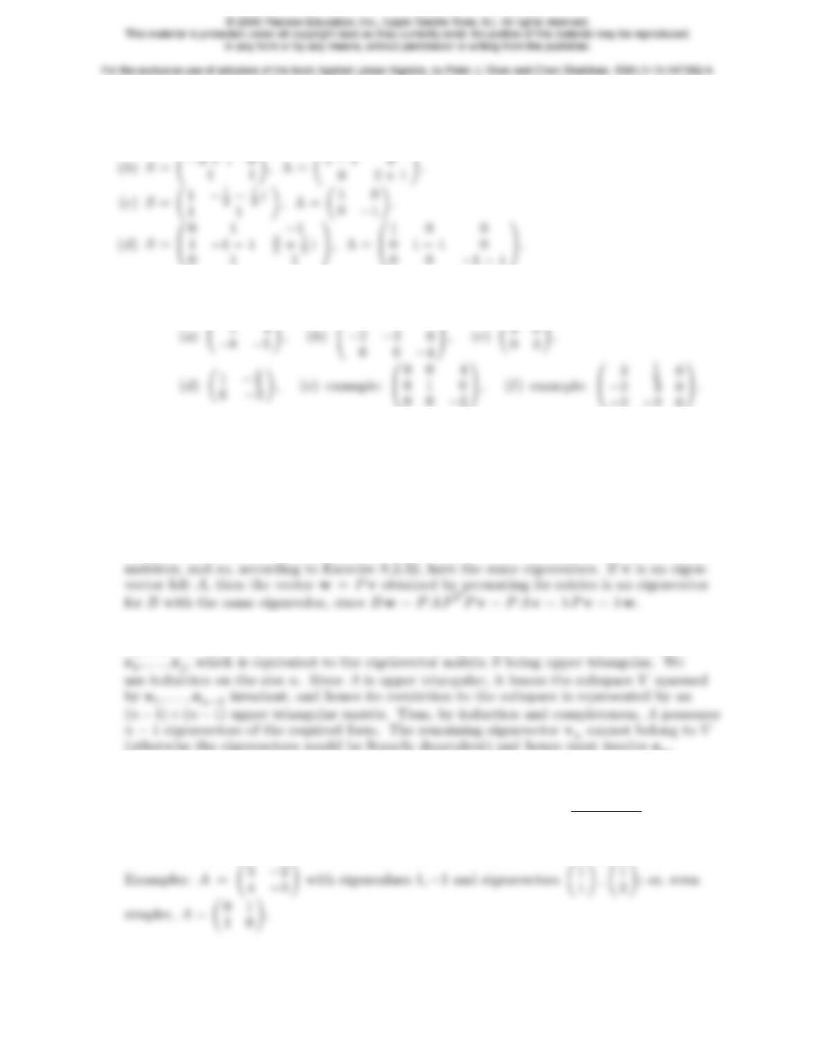
8.3.20. In all cases, A=SΛS−1.

(a)S= 1−1

1 1 !, Λ = 1 + i 0

0−1 + i !.

8.3.21. Use the formula A=SΛS−1. For parts (e,f ) you can choose any other eigenvalues and

eigenvectors you want to fill in Sand Λ.

6 6 −2

8.3.22. (a) 11 −6

18 −10 !, (b) −1 0

0 2 !, (c) −4−6

3 5 !.

♦8.3.23. Let S1be the eigenvector matrix for Aand S2the eigenvector matrix for B. Thus, by

the hypothesis S−1

1AS1= Λ = S−1

2B S2and hence B=S2S−1

1AS1S−1

2=S−1AS where

S=S1S−1

2.

8.3.24. The hypothesis says B=P AP T=P A P −1where Pis the corresponding permutation

matrix, and we are using Exercise 1.6.14 to identify PT=P−1. Thus Aand Bare similar

8.3.25. True. Let λj=ajj denote the jth diagonal entry of A, which is the same as the jth

eigenvalue. We will prove that the corresponding eigenvector is a linear combination of

8.3.26. The diagonal entries are all eigenvalues, and so are obtained from each other by permu-

tation. If all eigenvalues are distinct, then there are n! different diagonal forms — other-

wise, if it has distinct eigenvalues of multiplicities j1, . . . jk, there are n!

j1!··· jk!distinct

diagonal forms.

8.3.27. Let A=SΛS−1. Then A2= I if and only if Λ2= I , and so all its eigenvalues are ±1.

219

♥8.3.28.

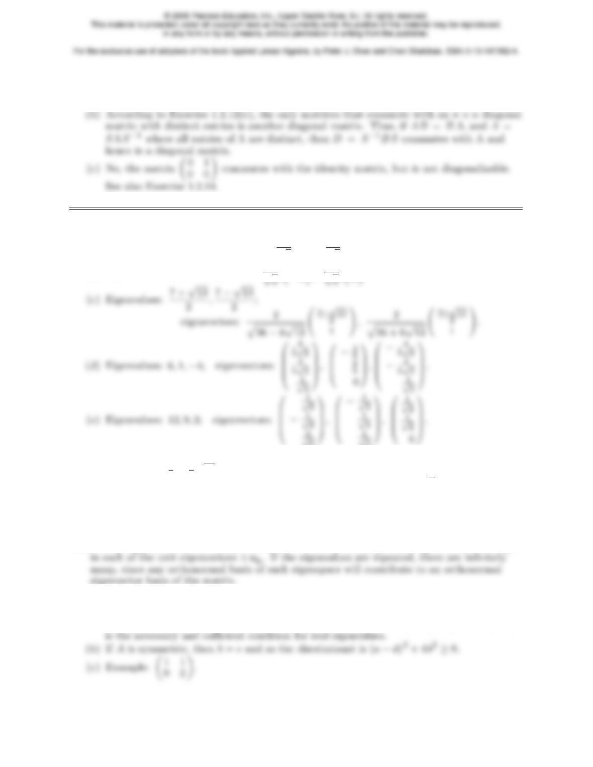
(a) If A=SΛS−1and B=S D S−1where Λ, D are diagonal, then AB =SΛD S−1=

S D ΛS−1=B A, since diagonal matrices commute.

8.4.1.

(a) Eigenvalues: 5,−10; eigenvectors: 1

√5 2

1!,1

√5 1

−2!.

(b) Eigenvalues: 7,3; eigenvectors: 1

√2 −1

√2 1

8.4.2.

(a) Eigenvalues 5

2±1

2√17; positive definite. (b) Eigenvalues −3,7; not positive definite.

(c) Eigenvalues 0,1,3; positive semi-definite. (d) Eigenvalues 6,3±√3; positive definite.

8.4.3. Use the fact that K=−Nis positive definite and so has all positive eigenvalues. The

eigenvalues of N=−Kare −λjwhere λjare the eigenvalues of K. Alternatively, mimic

the proof in the book for the positive definite case.

8.4.4. If all eigenvalues are distinct, there are 2ndifferent bases, governed by the choice of sign

8.4.5.

(a) The characteristic equation p(λ) = λ2−(a+d)λ+ (ad −bc) = 0 has real roots if and

only if its discriminant is non-negative: 0 ≤(a+d)2−4(a d −bc) = (a−d)2+ 4 bc, which

220

♥8.4.6.

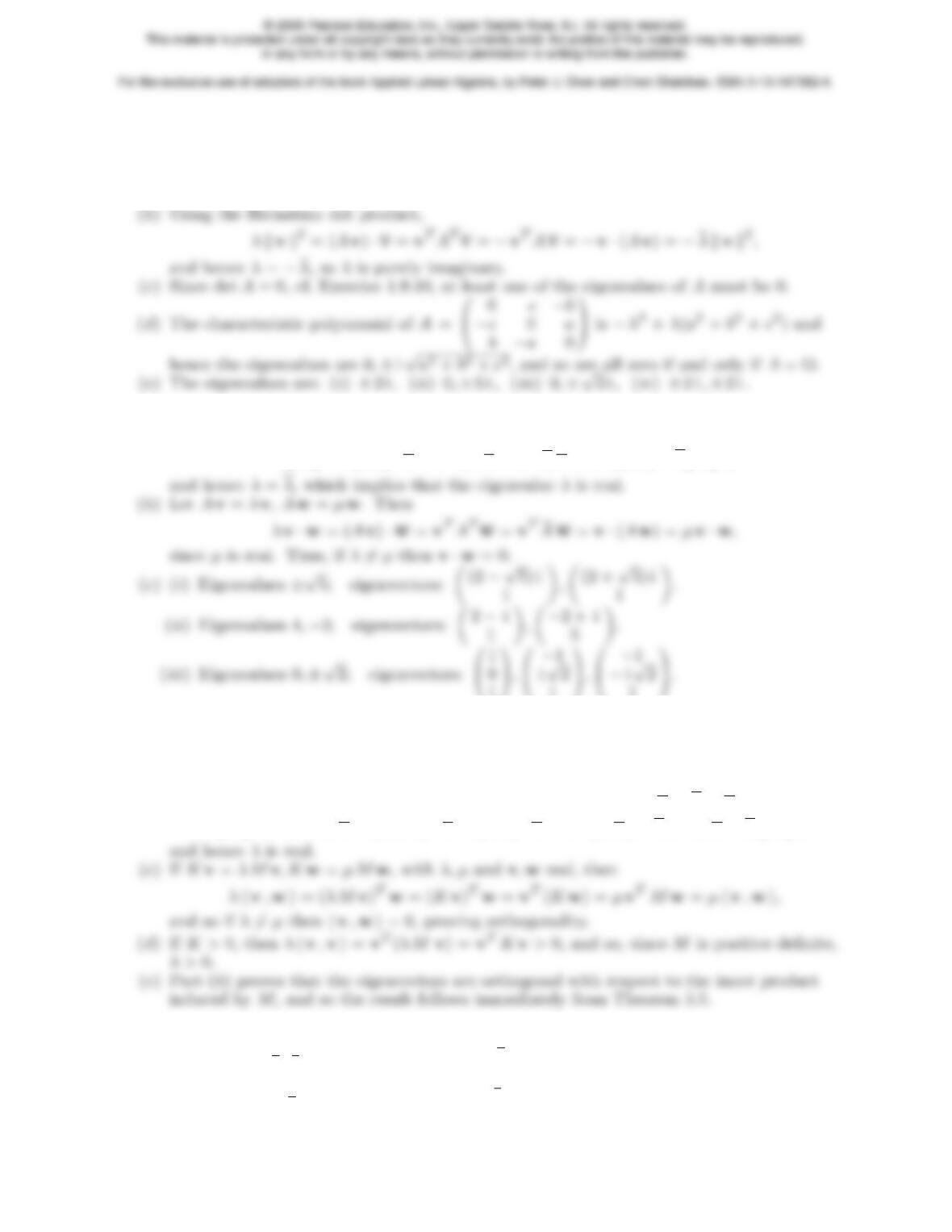
(a) If Av=λvand v6=0is real, then

λkvk2= (Av)·v= (Av)Tv=vTATv=−vTAv=−v·(Av) = −λkvk2,

and hence λ= 0.

♥8.4.7.

(a) Let Av=λv. Using the Hermitian dot product,

λkvk2= (Av)·v=vTATv=vTAv=v·(Av) = λkvk2,

11

♥8.4.8.

(a) Rewrite (8.31) as M−1Kv=λv, and so vis an eigenvector for M−1Kwith eigenvalue

λ. The eigenvectors are the same.

(b)M−1Kis not necessarily symmetric, and so we can’t use Theorem 8.20 directly. If vis

an generalized eigenvector, then since K, M are real matrices, Kv=λ M v. Therefore,

λkvk2=λvTMv= (λM v)Tv= (Kv)Tv=vT(Kv) = λvTMv=λkvk2,

8.4.9.

(a) Eigenvalues: 5

3,1

2; eigenvectors: −3

1!, 1

2

1!.

(b) Eigenvalues: 2,1

2; eigenvectors: 1

1!, −1

2

1!.

221