Chapter 7
7.1
// (1/)
0
() ( ) (ln ) ( )
11
80
y
y
y
ey
xx e
Gy PY y P X y PX e
e
edx e e
θθ θ
(1/ )
1
( ) for
8
y
ye
gy ee y
θ
7.3
2
2
2
0
() ( ) ( ) ( )
for 0 1
y
Gy PY y P X y PX y
dx y y
( ) 2 for 0 1gy y y
and 0 elsewhere
96 Mathematical Statistics, 8E
7.5
2
11 2 2
22 22 2 1
12
//
22
12
00
//()/
2
22
0
() ( ) ( )
11
11
yx
y
xx
y
xxyx
Gy PY y PX X y
eedxdx
eeedx
θθ
θθθ
θθ
θθ
7.6 (a)
() 0,Fy
(b)
2
1
() ,
2
Fy y
(c)
2
1
() 1 (2 ),
2
Fy y
(d)
() 1Fy
() 0, () , () 2 , () 0fy fy yfy yfy
7.7
1
12
() ( ) X
GZ PZ z P z
XX
xxzyz
Chapter 7 97
7.8
() 2
XY
PZ z P z
7.9
33 33
02 11
31 93
(0) , (1)
615 5 15 15 5
2
33
20 31
(2) 615 5
2
hh
h
7.10
X 0 1 2 Z 0 1
Z 1 0 1
()hz
3
5
2
5
98 Mathematical Statistics, 8E
7.13
X 2 3 4 5 6 7 8 9 10 11 12
()fx
1
36
2
36
3
36
4
36
5
36
6
36
5
36
4
36
3
36
2
36
1
36
(0)g
2541121
36 36 36 36 36 3
(1)g
363
36 36 36
12 1
36 3
(2)g
1452121
36 36 36 36 36 3
7.15
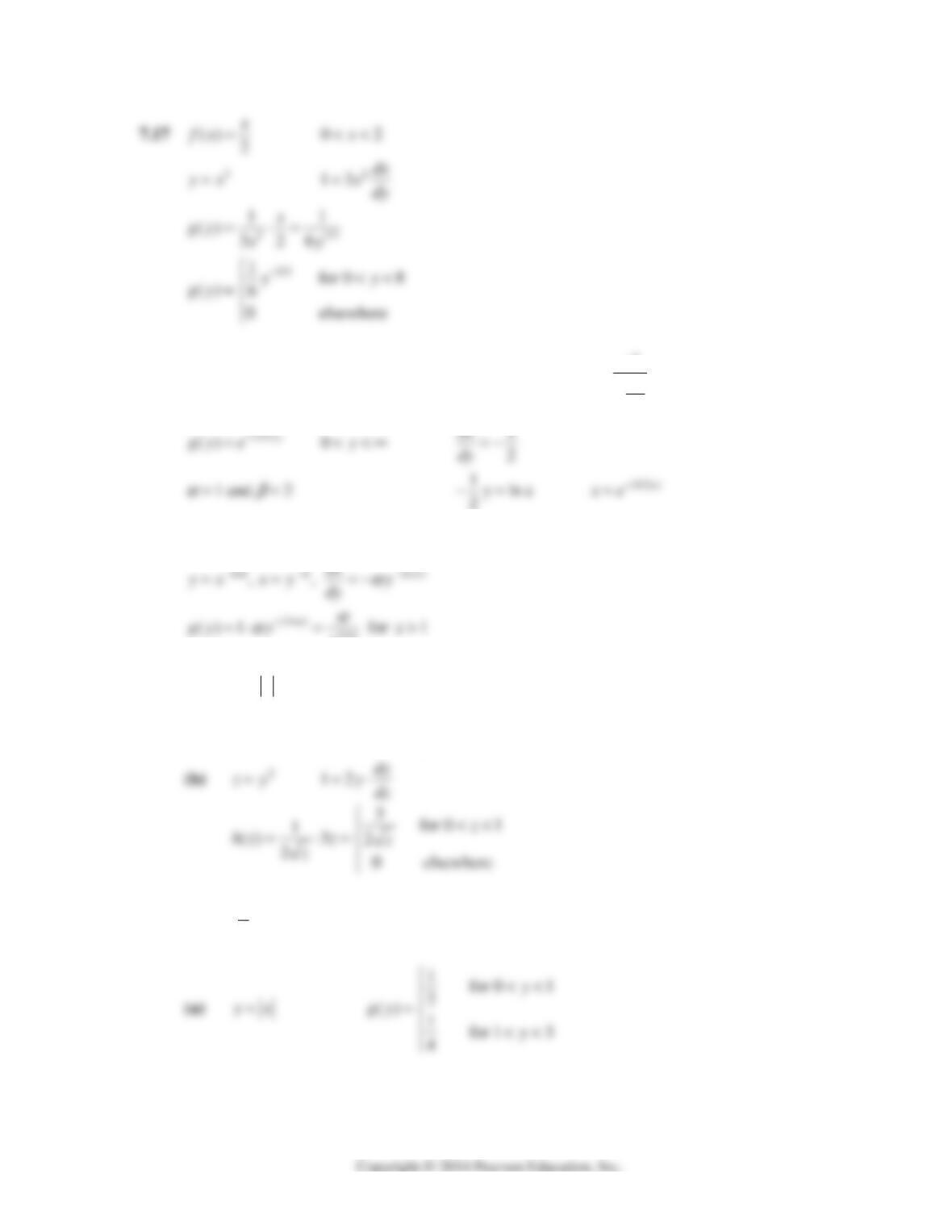
2
() 2
x
fx xe
2
yx
12
dx
xdy
2
for 0
1
() 2
20 elsewhere
y
x
ey
gy xe
x
Chapter 7 99
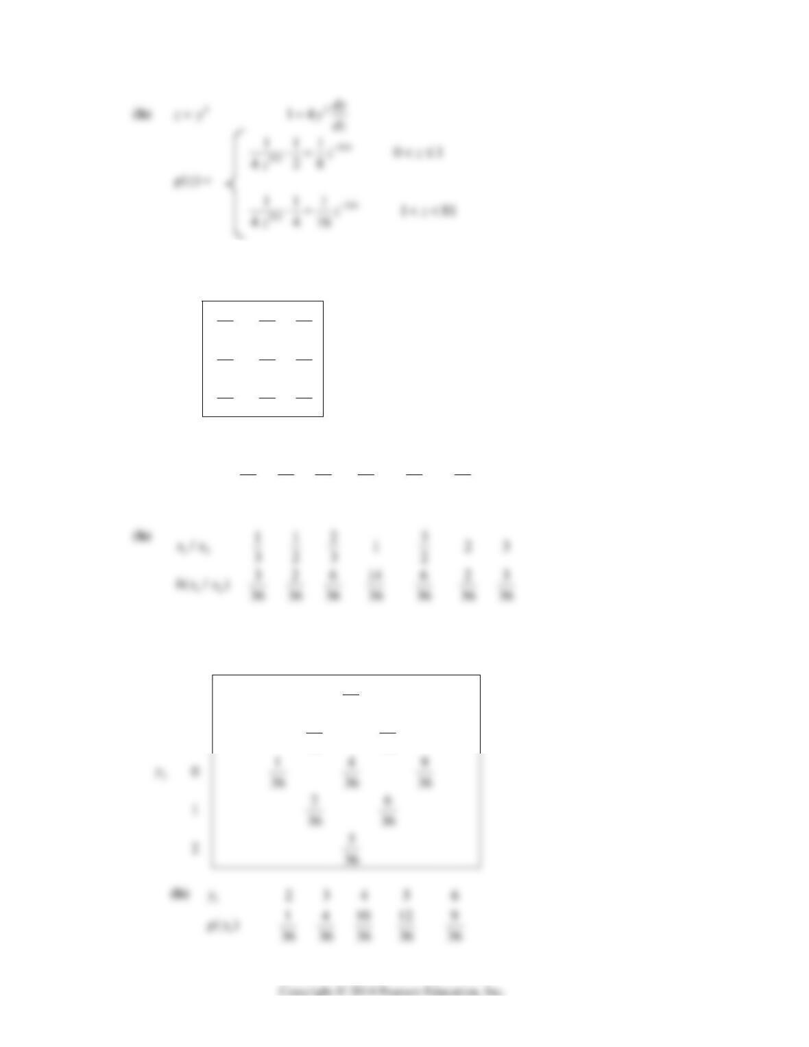
7.18
() 1fx
01x
2lnyx
2
1dx
xdy
7.19
() 1fx
01x
α
7.20 (a)
Yx
2
() () ( )
3 0 1
0 elsewhere
gy f y f y
yy
7.21
1
() 4
fx
1
α
3
β
100 Mathematical Statistics, 8E
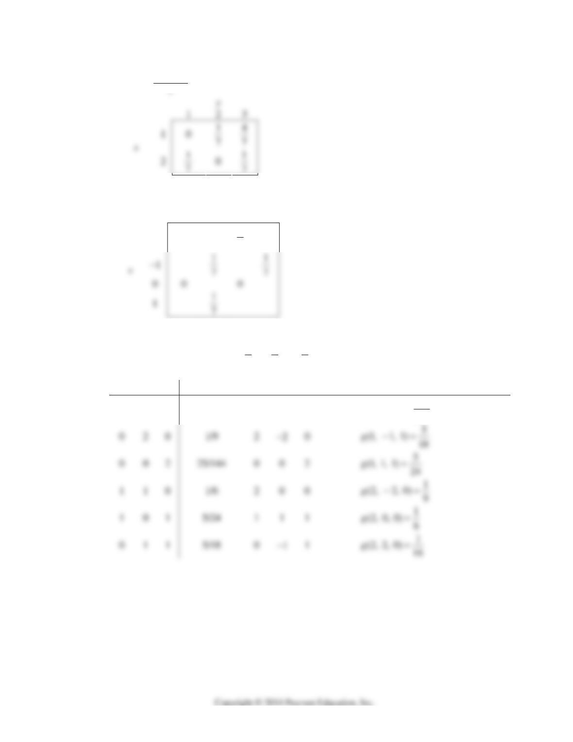
7.22
1
x
1 2 3
1
1
36
2
36
3
36
2
x
2
2
36
4
36
6
36
3
3
36
6
36
9
36
(a)
12
xx
1 2 3 4 6 9
12
()gxx
1
36
4
36
6
36
4
36
6
36
9
36
7.23 (a)
1
y
1 2 3 4 5 6
2
3
36
1
2
36
6
36
Chapter 7 101
7.24
2
()
(, ) 7
xy
fxy
1, 2x
1, 2, 3y
(a)
u
uxy
2 3 4 5
vxy
2
4
7
(b) u 2 3 4 5
()gu
0
2
7
4
7
1
7
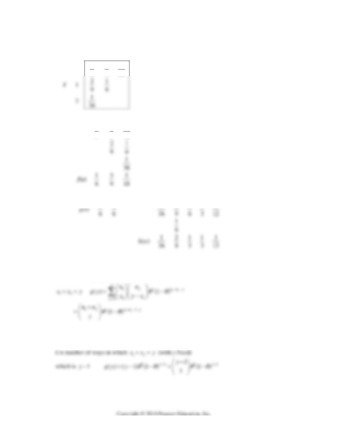
7.25
1
x
2
x
3
x
1
y
2
y
3
y
2 0 0 1/16 2 2 0
25
(0, 0, 2) 144
g
102 Mathematical Statistics, 8E
7.26
X
0 1 2
0
1
6
1
3
1
12
(a) u 0 1 2
1
6
1
3
1
12
(b) v 0 1 w
2
1
0 1 2
g(v)
5
1
1
2
1
1
1
7.27
12 12 12
12 ()
12
12
(, ) (1 )
xx nn xx
nn
fxx xx
θθ
7.28
12
11
12 1 2
( , ) (1 ) (1 )
xx
fxx x x y
θθθθ
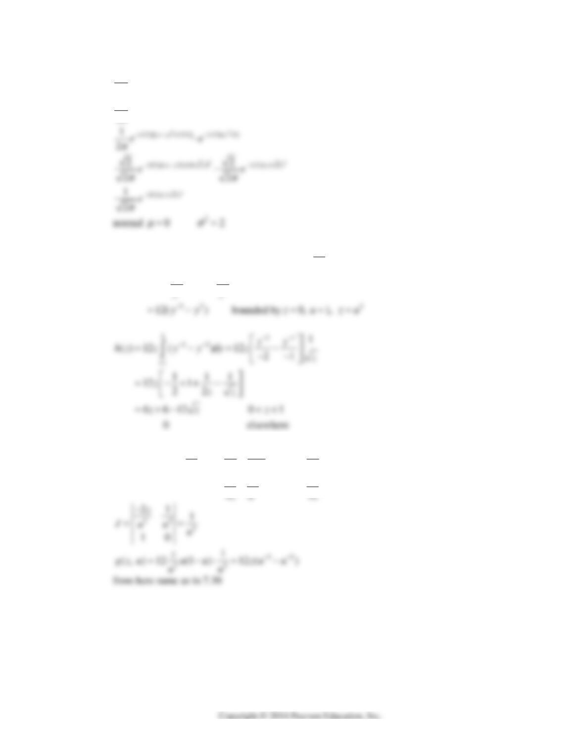
22 22
( ) (1 ) * ( ; 2, ) ( 1) (1 )
yy
gy k b y y
θθ θ θθ
Chapter 7 103
7.29
22
(1/2)( )
1
2
xy
ezxy
π
22
(1/2)[ ( ) ]
1
2
xzx
e
π
7.30
22
( , ) 12 (1 ) 1 dx
fxy xy y z xy y
dz
22
1
(, ) 12 (1 )
z
gz y y
yy
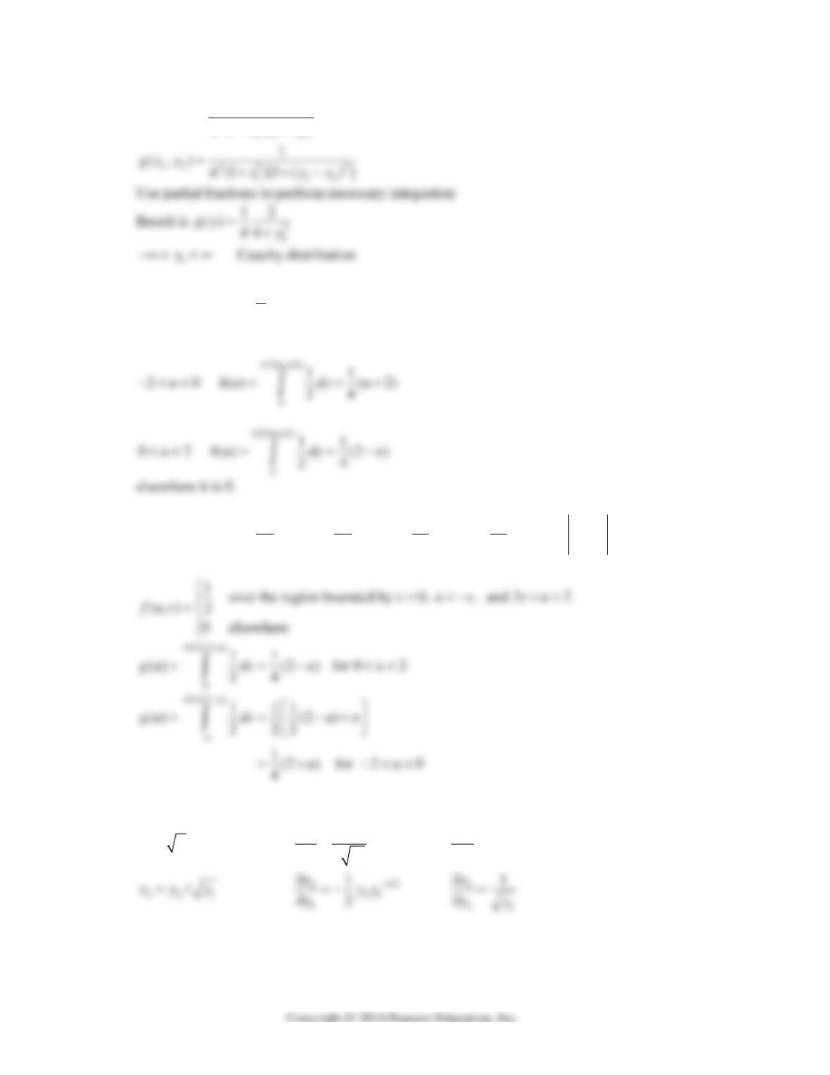
7.31
2
zxy
2
z
xu
2
2xz
uu
1
y
u
uy
yu
2
1x
0
y
104 Mathematical Statistics, 8E
7.32
12 1 2
22 2
1
( , )
(1 )(1 )
fx x y x x
xx
π
7.34
(, )gu y
1 over region bounded by 0, , and 2 0
2yuy yu
0 elsewhere
7.35
, uyxvx
1
u
x
1
u
y
1
v
x
0
v
y
11 1
10
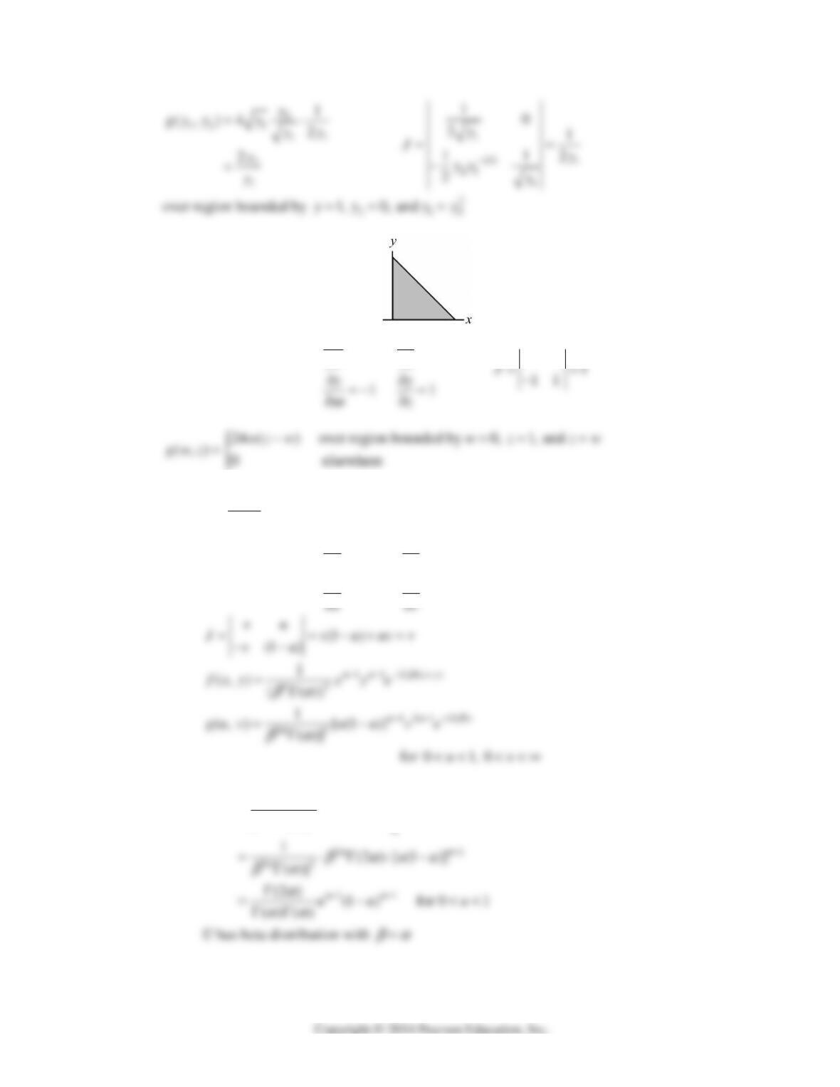
7.36
12 12
(, ) 4fx x xx
2
11
yx
212
yxx
1
xy
1
11
1
2
x
yy
1
2
0
x
y
Chapter 7 105
7.37
(, ) 24fxy xy
zxywx xw
and
yzw
1 0
xx
wz
10 1
7.38 (a)
and
x
uvxy
xy
xuv
xv
u
xu
v
(1 )
yv u
yv
1
yu
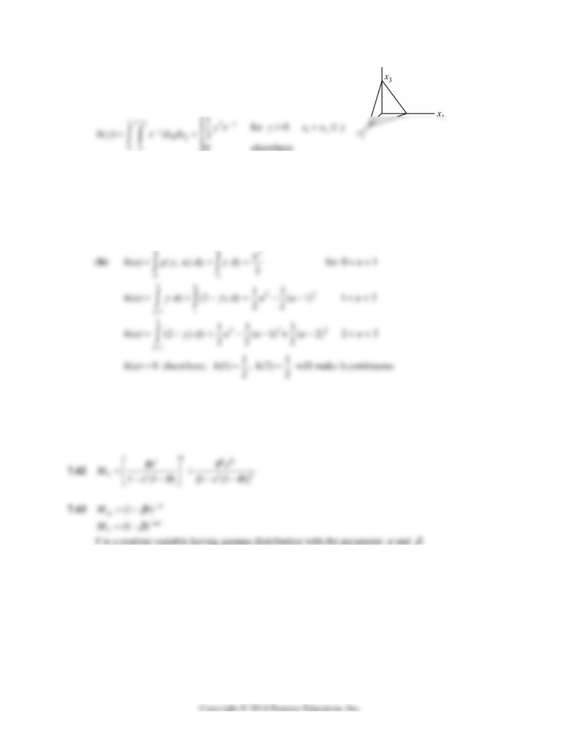
(b)
121(1/)
22
1
() [(1 )]
()]
v
hu u u v e dv
ααβ
α
βα
Γ
106 Mathematical Statistics, 8E
7.39
123
yx x x
12
(, , )
y
gx x y e
12
0, 0, 0xxy
7.40
3
(, ) ()gyx hy
as given in Example 7.13
(a)
I II
( , ) ( ) 1 2 III IV
0 elsewhere
y
gyu hy y
7.41
12
12
[1 ( 1) [1 ( 1)]
[1 ( 1)]
nntt
Y
nnt
Me e
e
θθ
θ
Y is random variable having binomial distribution with the parameter
θ
and
12
nn
.
7.44
22
(1/2)tt
X
Me
μ
σ
22
22
(1/2)
(1/2)
ii
ii
tt
tt
Y
Me e
μ
σ
μσ
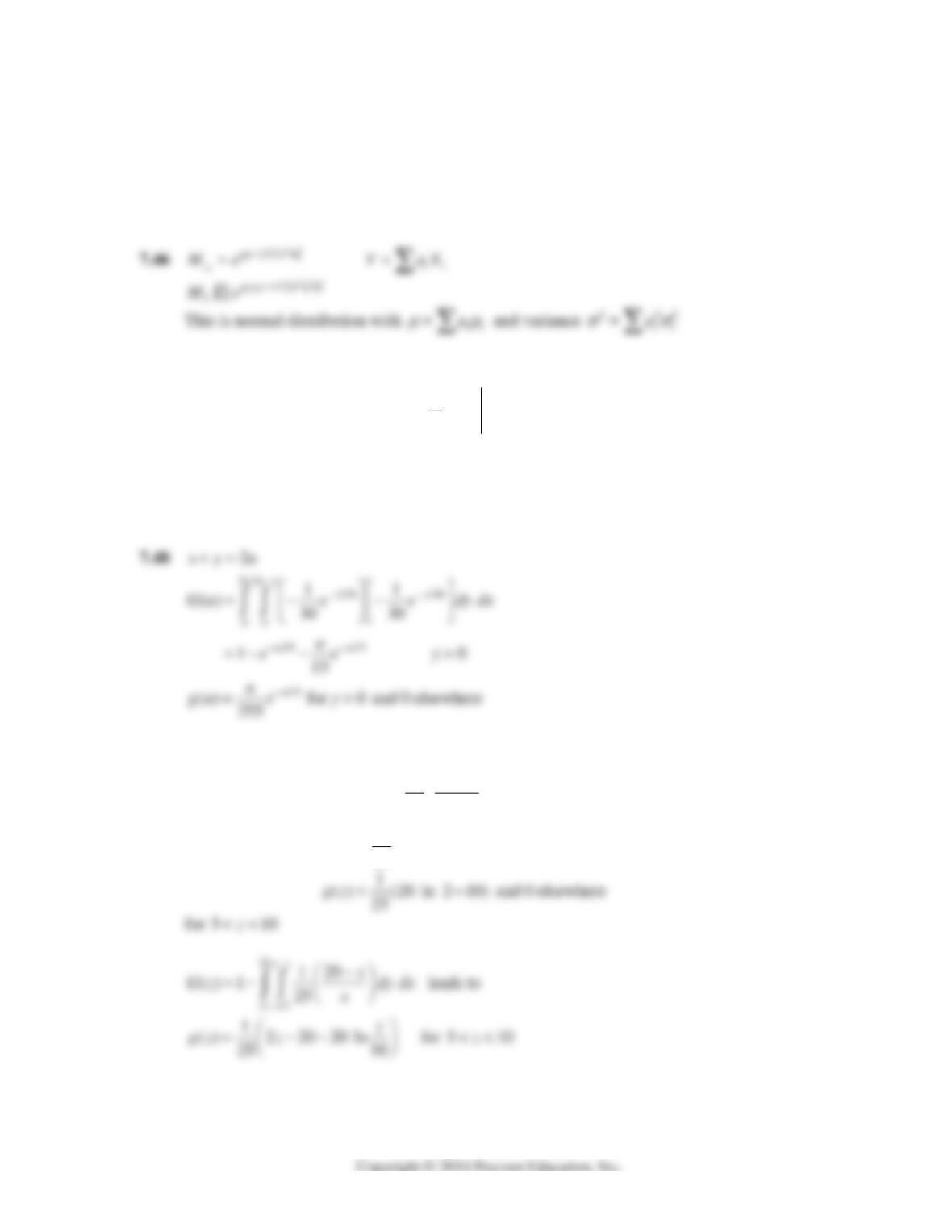
Y is a random variable having normal distribution with
2
and
i
μ
μσ
2
i
σ
Chapter 7 107
7.45 Let
iii
Z
aX
()
ii
Z
xi
MMat
since
i
YZ
( ) QED
i
Yxi
MMat
7.47
/
0.4 0.4
0.2 0 0.2
0.4
0.2
() ( ) ( )
/
1
5 5 0
5[1 ] 1
vp
sp sp
vv
Gv PV v PSP v
vp
p e ds dp p e dp
p
edp e
( ) for 0
v
gv e v
and 0 elsewhere
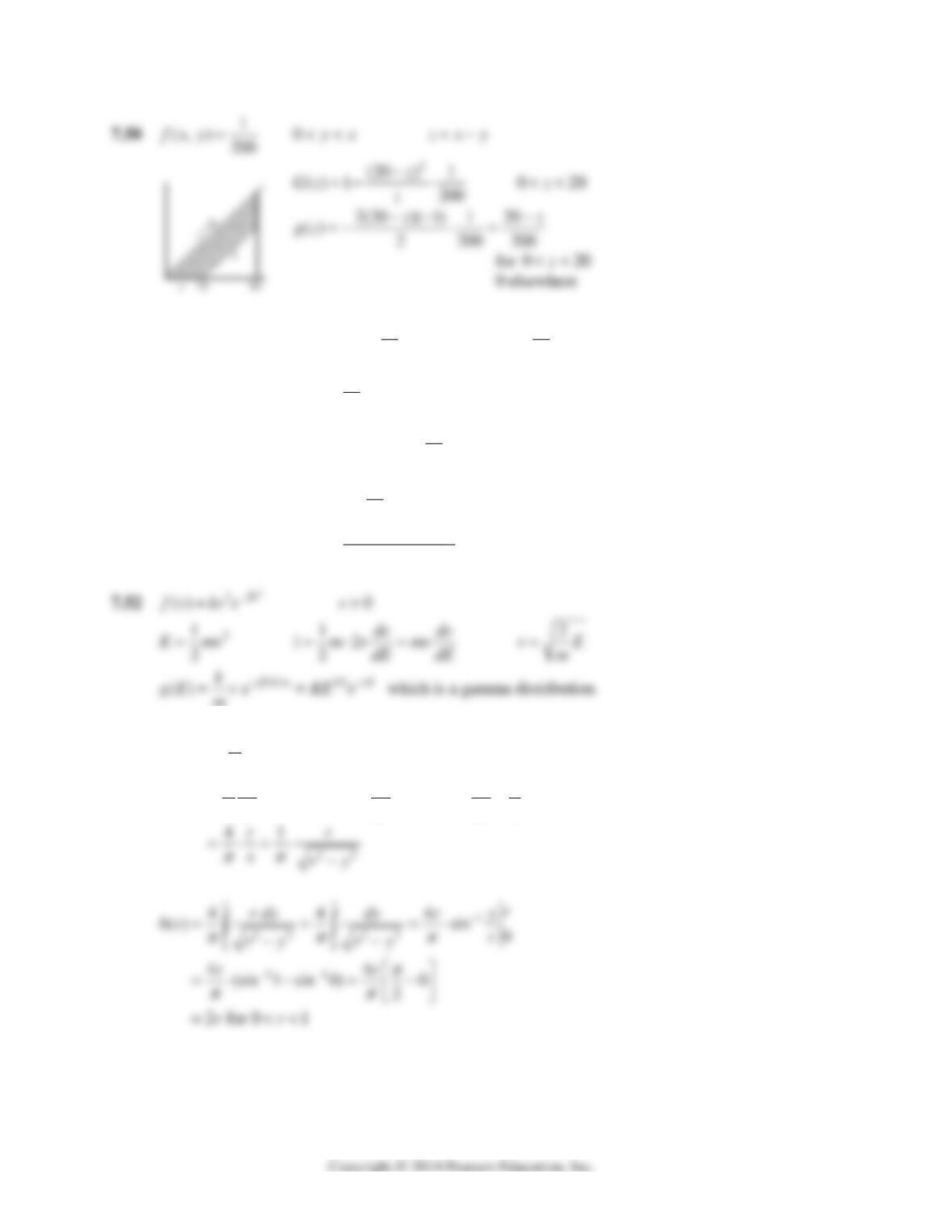
7.49
zxy
for
05z
20
10
120
()
25
1(20 ln 2 10)
25
x
xz
x
G z dy dx
x
z
108 Mathematical Statistics, 8E
7.51 for
01y
1
3
1221
00
33
() (5 )
11 11
yx
y
G y x x dx dx y
2
9
() 11
gy y
for
12y
2
2
2(1 )
2
1212
0
2
3
() 1 (5 )
11
1
1(17)(2)
11
x
y
yx
G y x x dx dx
yy
3(2 )(7 4)
() 11
yy
gy
m
7.53
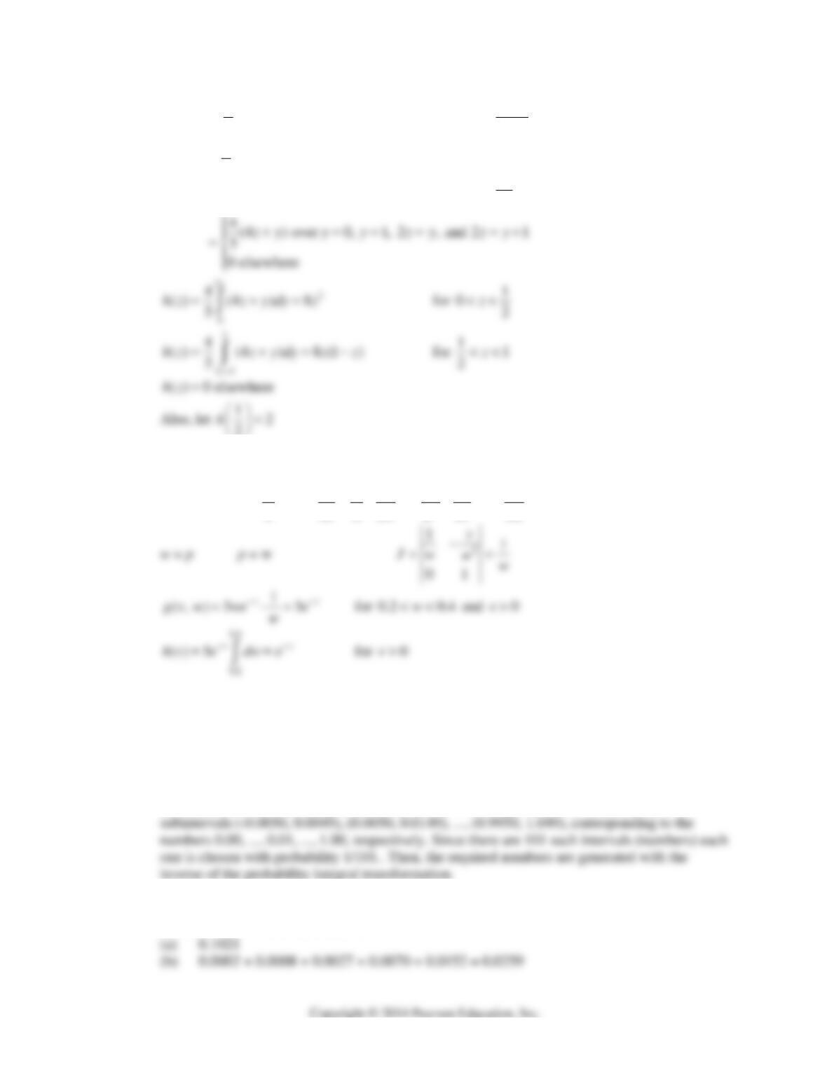
1
(, )fxy
π
22
01xy
222
rxy
4
(, ) dx
gry dr
π
2dx
rdr
dx r
dr x
Chapter 7 109
7.54
2
(, ) (2 3)
5
fxy x y
01
01
x
y
xy
zz
2
(, ) [4 ]2
5
gz y z y
2zxy
dx
zdz
7.55
(, ) 5
ps
fps pe
0.2 0.4p
and
0s
vsp
v
sw
2
1, , 0, 1
ssvpp
vw w v w
w
7.56 Using MINITAB, we generate 10 “pseudo-random” numbers in C1 having the standard normal
distribution with the following commands:
MTB> Random 10 C1
SUBC> Normal 0.0 1.0.
7.57 First the computer generates 10 “pseudo-random” numbers on the interval (0, 1). For example,
for numbers to two decimal places, the interval (0, 1) is regarded as the union of the
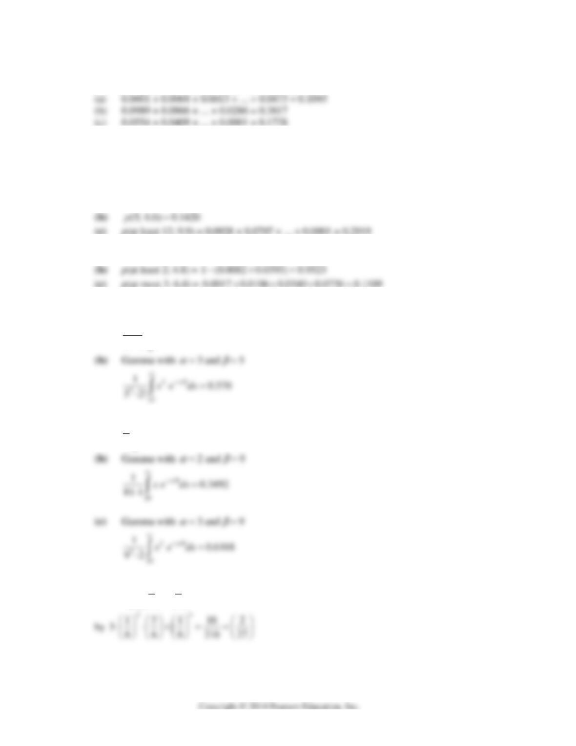
7.58 Total number of calls per hour is random variable having Poisson distribution with parameter
2.1 10.9 13.
λ
From Table II
110 Mathematical Statistics, 8E
7.59 Total number of inquiries is a random variable having Poisson distribution with
3.6 5.8 4.6 14.
λ
From Table II
7.60 Six inquiries with
2
5.8
λ
(6; 5.8) 0.1601p
Table ii
Eight inquiries with
8.2
λ
(8; 8.2) 0.1392p
(0.1601)(0.1392) 0.0222
7.61 (a)
(2; 3.3) 0.2008p
7.62 (a)
(4; 3.2) 0.1781p
7.63 (a) Gamma with
2 and 5
αβ
8
/5
2
1 0.475
51
x
txe dx
7.64 (a)
/9 20/9 2.22
20
10.1086
9
x
edxe e
7.65
3
315
() , 0, 1, 2, 3.
66
xx
fx x
x
For
22, 1xx
. The probability that
1x
is given
Chapter 7 111
7.67 (a)
6
0
12
12.5,
55
ddd k
k
.
(b)
22.
dA
Ad
ππ
Thus,
1/2
21
;
dA
dA d dd dd A dA
π
.
7.69
22
()/2
1
() 2
x
fx e
μ
σ
πσ
. Substituting
lnyx
, with
y
xe
and
y
dx e dy
, we obtain
22
1(ln )/2
1
() 2
y
gy y e
μ
σ
πσ
for
0y
, and
() 0gy
elsewhere.