Solutions — Chapter 7
7.1.1. Only (a) and (d) are linear.
7.1.3. (a)F(0,0) = 2
0!6= 0
0!, (b)F(2x, 2y) = 4F(x, y)6= 2F(x, y), (c)F(−x, −y) =
7.1.5. (a)0
B
@
0−1 0
1 0 0
0 0 1 1
C
A, (b)0
B
B
B
@
1 0 0
01
2−√3
2
1
C
C
C
A, (c)0
B
@
1 0 0
0 1 0
0 0 −11
C
A, (d)0
B
@
0 0 1
100
0 1 0 1
C
A,
7.1.6. L x
y!=5
2x−1
2y. Yes, because 1
1!, 1
−1!form a basis, so we can write any v∈
7.1.7. L(x, y) = 0
@−2
3x+4
3y
−1
3x−1
3y1
A.
7.1.8. The linear function exists and is unique if and only if x1
y1!, x2
y2!are linearly indepen-
7.1.9. No, because linearity would require
matrix representative: 0
B
@
0−c b
c0−a
−b a 01
C
A.
7.1.11. No, since N(−v) = N(v)6=−N(v).
7.1.14.
(a)L[cX +dY ] = A(cX +dY ) = cAX +dAY =c L[X] + d L[Y];
matrix representative: 0
B
B
B
@
a0b0
0a0b
c0d0
1
C
C
C
A.
7.1.15. (a) Linear; target space = Mn×n. (b) Not linear; target space = Mn×n.
(c) Linear; target space = Mn×n. (d) Not linear; target space = Mn×n.
(e) Not linear; target space = R. (f) Linear; target space = R. (g) Linear; target space =
Rn. (h) Linear; target space = Rn. (i) Linear; target space = R.
♦7.1.16. (a) If Lsatisfies (7.1), then L[cv+dw] = L[cv] + L[dw] = c L[v] + d L[w], proving
♦7.1.17. If v=c1v1+··· +cnvn, then, by linearity,
♥7.1.18.
(a)B(cv+e
ce
v,w) = (cv1+e
ce
v1)w1−2(cv2+e
ce
v2)w2=c(v1w1−2v2w2)+e
c(e
v1w1−2e
v2w2) =
cB(v,w) + e
cB(e
v,w),so B(v,w) is linear in vfor fixed w. Similarly, B(v, cw+e
ce
w) =
177
(d)B(cv+e
ce
v,w) = (cv+e
ce
v)TAw=cvTAw+e
ce
vTAw=cB(v,w) + e
cB(e
v,w),
7.1.19. (a) Linear; target space = R. (b) Not linear; target space = R. (c) Linear; target
space = R. (d) Linear; target space = R. (e) Linear; target space = C1(R). (f) Linear;
7.1.20. True. For any constants c, d,
7.1.21.
Mh[cf(x) + dg(x)] = h(x) (c f (x) + d g(x)) = c h(x)f(x) + d h(x)g(x) = cMh[f(x)]+dMh[g(x)].
To show the target space is Cn[a, b ], you need the result that the product of two ntimes
continuously differentiable functions is ntimes continuously differentiable.
7.1.26.
(a) Gradient: ∇(cf +dg) = c∇f+d∇g; domain is space of continuously differentiable
scalar functions; target is space of continuous vector fields.
7.1.27.
(a) dimension = 3; basis: ( 1,0,0 ) ,( 0,1,0 ) ,( 0,0,1 ).
(b) dimension = 4; basis: 1 0
0 0 !, 0 1
0 0 !, 0 0
1 0 !, 0 0
0 1 !.
7.1.28. True. The dimension is 2, with basis 0 1
0 0 !, 0 0
0 1 !.
7.1.29. False. The zero function is not an element.
−1!, (ii )a= 3 0
0 2 !−1 2
−1!= 2
−1!, (iii )a= 2−1
−1 3 !−1 2
−1!= 1
0!.
♥7.1.32.
(a) By linearity, Li[x1v1+··· +xnvn] = x1Li[v1] + ···+xnLi[vn] = xi.
(b) Every real-valued linear function L∈V∗has the form L[v] = a1x1+··· +anxn=
179
7.1.33. In all cases, the dual basis consists of the liner functions Li[v] = riv. (a)r1=
“1
2,1
2”,r2=“1
2,−1
2”, (b)r1=“1
7,3
7”,r2=“2
7,−1
7”, (c)r1=“1
2,1
2,−1
2”,r2=
“1
2,−1
2,1
2”,r3=“−1
2,1
2,1
2”, (d)r1= ( 8,1,3 ) ,r2= ( 10,1,4 ) ,r3= ( 7,1,3 ),
(e)r1= ( 0,1,−1,1 ) ,r2= ( 1,−1,2,−2 ) ,r3= ( −2,2,−2,3 ) ,r4= ( 1,−1,1,−1 ).
7.1.37.
(a)S◦T=T◦S= clockwise rotation by 60◦= counterclockwise rotation by 300◦;
(b)S◦T=T◦S= reflection in the line y=x;
(c)S◦T=T◦S= rotation by 180◦;
7.1.38. (a)L= 1−1
−3 2 !; (b)M= −1 0
−3 2 !; (c)N= 2 1
0 1 !;
7.1.39. (a)R=0
B
@
1 0 0
0 0 −1
0 1 0 1
C
A,S=0
B
@
0−1 0
1 0 0
0 0 1 1
C
A; (b)R◦S=0
B
@
0−1 0
0 0 −1
1001
C
A6=S◦R=
0
B
@
0 0 1
100
0 1 0 1
C
A; under R◦S, the basis vectors e1,e2,e3go to e3,−e1,−e2, respectively.
180
nal projection onto L=8
>
<
>
:t0
B
@
1
0
11
C
A9
>
=
>
;has matrix representative M=0
B
B
@
1
201
2
0 0 0
1
201
2
1
C
C
A6=R.
7.1.41. (a)L=E◦Dwhere D[f(x)] = f′(x), E[g(x) ] = g(0). No, they do not commute
—D◦Eis not even defined since the target of E, namely R, is not the domain of D, the
space of differentiable functions. (b)e= 0 is the only condition.
♦7.1.44. (a) Given L:V→U,M:W→Vand N:Z→W, we have, for z∈Z,
((L◦M)◦N)[z] = (L◦M)[N[z]] = L[M[N[z]]] = L[(M◦N)[z]] = (L◦(M◦N))[ z]
as elements of U. (b) Lemma 7.11 says that M◦Nis linear, and hence, for the same rea-
son, (L◦M)◦Nis linear. (c) When U=Rm,V=Rn,W=Rp,Z=Rq, then Lis
represented by an m×nmatrix A,Mis represented by a n×pmatrix B, and Nis repre-
sented by an p×qmatrix C. Associativity of composition implies (AB)C=A(B C).
♥7.1.47.
(a) Both L◦Mand M◦Lare linear by Lemma 7.11, and, since the linear transformations
form a vector space, their difference L◦M−M◦Lis also linear.
(b)L◦M=M◦Lif and only if [ L, M ] = L◦M−M◦L= O.
(c) (i) 1 3
0−1!, (ii ) 0−2
−2 0 !, (iii )0
B
@
0 2 0
−2 0 −2
0 2 0 1
C
A.
(d)h[L, M ], N i= (L◦M−M◦L)◦N−N◦(L◦M−M◦L)
=L◦M◦N−M◦L◦N−N◦L◦M+N◦M◦L,
181
♦7.1.48.
(a) [ P, Q ] [f] = P◦Q[f]−Q◦P[f] = P[x f ]−Q[f′] = (xf)′−xf′=f.
(b) According to Exercise 1.2.32, the trace of any matrix commutator is zero: tr[ P, Q ] = 0.
On the other hand, tr I = n, the size of the matrix, not 0.
♥7.1.49.
(a)D(1) is a subspace of the vector space of all linear operators acting on the space of poly-
independent.
(b) If L=p(x)D+q(x) and M=r(x)D+s(x), then
L◦M=pr D2+ (pr′+q r +p s)D+ (p s′+q s),
7.1.51. (a) The inverse is the scaling transformation that halves the length of each vector.
(b) The inverse is counterclockwise rotation by 45◦.
7.1.52.
(a) Function: 2 0
20
7.1.53. Since Lhas matrix representative 1 3
−1−2!, its inverse has matrix representative
−1 1 2 1
182
−1 1 −1
−1
−1
♦7.1.55. If L◦M=L◦N= I W, M ◦L=N◦L= I V,then, by associativity,
M=M◦IW=M◦(L◦N) = (M◦L)◦N= I V◦N=N.
♥7.1.56.
(a) Every vector in Vcan be uniquely written as a linear combination of the basis elements:
v=c1v1+···+cnvn. Assuming linearity, we compute
L[v] = L[c1v1+··· +cnvn] = c1L[v1] + ··· +cnL[vn] = c1w1+··· +cnwn.
(b) The inverse is uniquely defined by the requirement that L−1[wi] = vi,i= 1, . . . , n.
Note that L◦L−1[wi] = L[vi] = wi, and hence L◦L−1= I Wsince w1, . . . , wnis a
basis. Similarly, L−1◦L[vi] = L−1[wi] = vi, and so L−1◦L= I V.
(c) If A= ( v1v2. . . vn), B= ( w1w2… wn), then Lhas matrix representative B A−1,
while L−1has matrix representative AB−1.
7.1.57. Let m= dim V= dim W. As guaranteed by Exercise 2.4.24, we can choose bases
v1,…,vnand w1,…,wnof Rnsuch that v1,…,vmis a basis of Vand w1, . . . , wmis
a basis of W. We then define the invertible linear map L:Rn→Rnsuch that L[vi] = wi,
i= 1, . . . , n, as in Exercise 7.1.56. Moreover, since L[vi] = wi,i= 1, . . . , m, maps the basis
of Vto the basis of W, it defines an invertible linear function from Vto W.
♦7.1.59. Use associativity of composition: N=N◦IW=N◦L◦M= I V◦M=M.
7.1.60.
(a)L[ax2+bx +c] = ax2+ (b+ 2a)x+ (c+b);
♥7.1.61.
(a) It forms a three-dimensional subspace since it is spanned by the linearly independent
functions x2ex, xex, ex.
7.2.1.
(a)0
B
@
1
√2−1
√2
1
√2
1
√2
1
C
A. (i) The line y=x; (ii ) the rotated square 0 ≤x+y, x −y≤√2;
(iii ) the unit disk.
( 1,3 )T,( 0,1 )T; (iii ) the elliptical domain 5x2−4xy +y2≤1.
(e)0
@−1
23
2
−3
25
21
A=0
B
@
1
√2−1
√2
1
√2
1
√2
1
C
A 1 3
0 1 !0
B
@
1
√2
1
√2
−1
√2
1
√2
1
C
A.
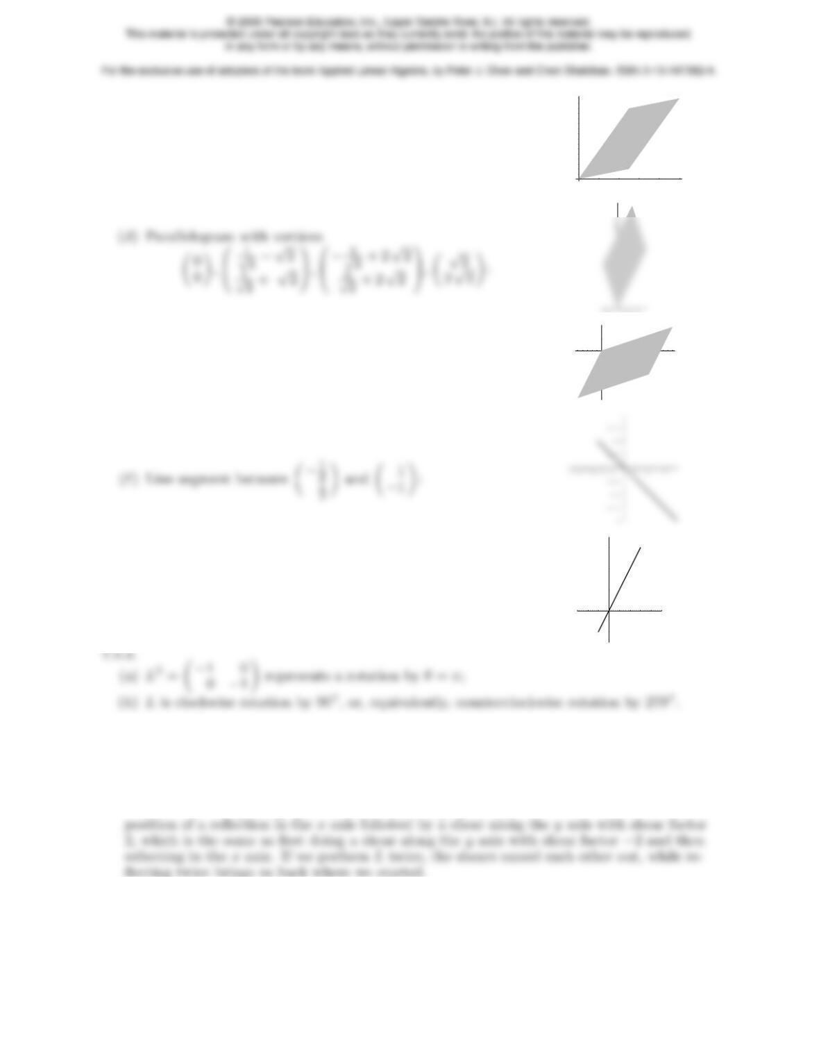
7.2.2. Parallelogram with vertices 0
0!, 1
2!, 4
3!, 3
1!:
12 3 4
0.5
1
1.5
2
2.5
3
-2
4
(c) Parallelogram with vertices 0
0!, 5
7!, 10
8!, 5
1!:
246 8 10
2
4
6
8
-0.5 0.5 1
5
(e) Parallelogram with vertices 0
0!, 3
1!, 2
−1!, −1
−2!:
-1 1 2 3
-2
-1.5
-1
-0.5
0.5
1
(g) Line segment between −1
−2!and 3
6!:
-3 -2 -1 1 2 3 4 5
-2
2
4
6
7.2.4. 0 1
1 0 !2
= 1 0
0 1 !.Lrepresents a reflection through the line y=x. Reflecting twice
brings you back where you started.
7.2.5. Writing A= 1 0
2 1 ! 1 0
0−1!= 1 0
0−1! 1 0
−2 1 !, we see that it is the com-
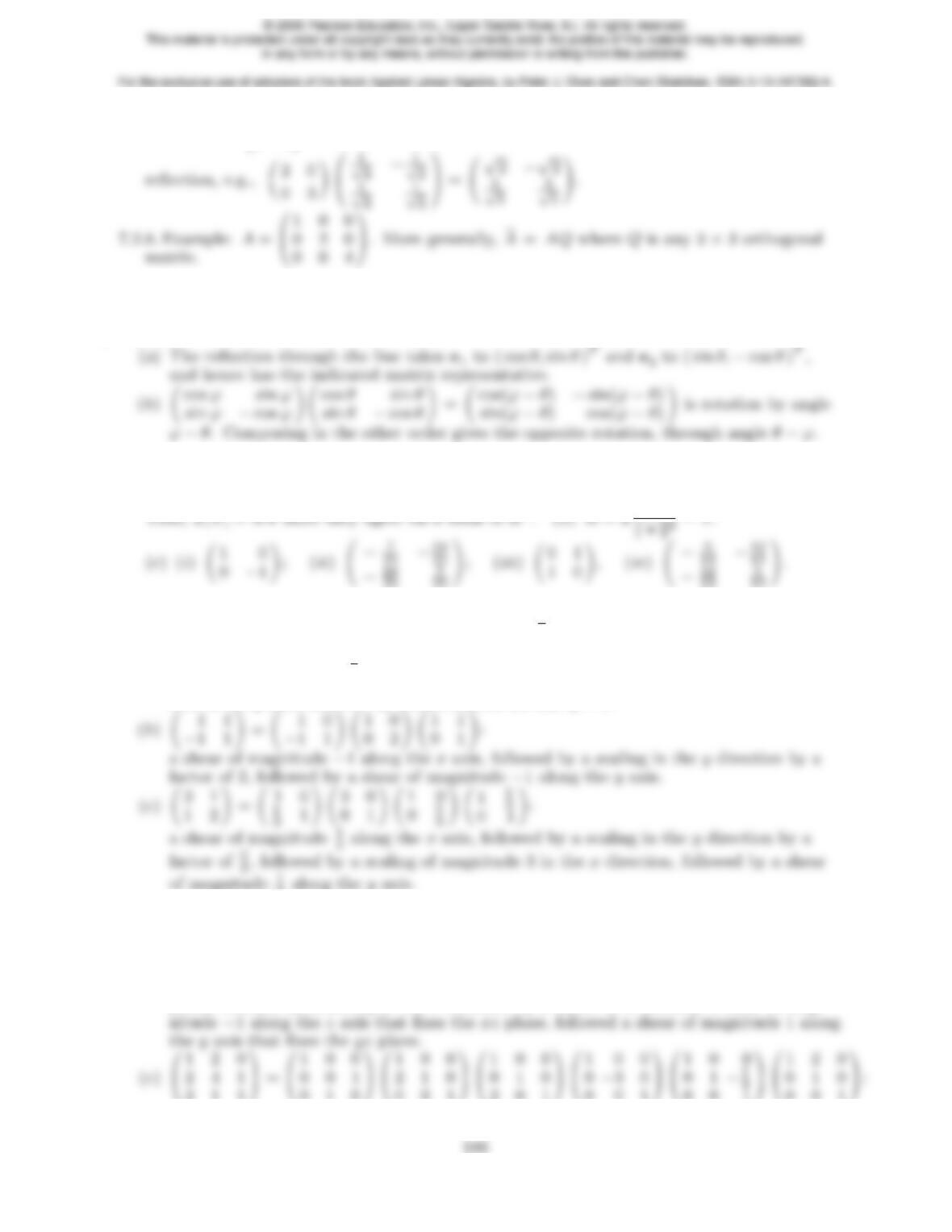
7.2.6. Its image is the line that goes through the image points −1
2!, −4
−1!.
185
7.2.7. Example: 2 0
0 3 !. It is not unique, because you can compose it with any rotation or
7.2.9. (a) True. (b) True. (c) False: in general, squares are mapped to parallelograms. (d) False:
in general circles are mapped to ellipses. (e) True.
♦7.2.10.
♦7.2.11. (a) Let zbe a unit vector that is orthogonal to u, so u,zform an orthonormal basis of
R2. Then L[u] = u=Rusince uTu= 1, while L[z] = −z=Rzsince u·z=uTz= 0.
7.2.12.
(a) 0 2
−3 1 != 0 1
1 0 ! −3 0
0 1 ! 1 0
0 2 ! 1−1
3
0 1 !:
a shear of magnitude −1
3along the xaxis, followed by a scaling in the ydirection by a
factor of 2, followed by a scaling in the xdirection by a factor of 3 coupled with a reflec-
tion in the yaxis, followed by a reflection in the line y=x.
3along the yaxis.
(d)0
B
@
110
1 0 1
0111
C
A=0
B
@
100
1 1 0
0011
C
A0
B
@
1 0 0
0 1 0
0−1 1 1
C
A0
B
@
1 0 0
0 1 0
0 0 2 1
C
A0
B
@
1 0 0
0−1 0
0 0 1 1
C
A0
B
@
1 0 0
0 1 −1
0 0 1 1
C
A0
B
@
1 1 0
0 1 0
0 0 1 1
C
A:
a shear of magnitude 1 along the xaxis that fixes the xz plane, followed a shear of mag-
nitude −1 along the yaxis that fixes the xy plane, followed by a reflection in the xz
plane, followed by a scaling in the zdirection by a factor of 2, followed a shear of mag-
2 1 1 1
0 1 0 1
0 0 1 1
2 0 1 1
0 0 1 1
0 0 1 1
0 0 1 1
7.2.13.
(a) 1a
0 1 ! 1 0
b1! 1a
0 1 != 1 + ab 2a+a2b
b1 + ab != cos θ−sin θ
sin θcos θ!since
7.2.14. 0
B
B
@
1 0 0
01
2−√3
2
0√3
21
2
1
C
C
A=0
B
@
1 0 0
0 1 0
0√3 1 1
C
A0
B
@
1 0 0
01
20
0 0 1 1
C
A0
B
@
1 0 0
0 1 0
0 0 2 1
C
A0
B
@
1 0 0
0 1 −√3
0 0 1 1
C
A:
a shear of magnitude −√3 along the yaxis that fixes the xy plane, following by a scaling
in the zdirection by a factor of 2, following by a scaling in the ydirection by a factor of 1
2,
following by a shear of magnitude √3 along the zaxis that fixes the xz plane.
7.2.15. (a) 1 0
0 0 !, (b)0
@
1
21
2
1
21
21
A, (c)0
@
4
13 −6
13
−6
13 9
13 1
A.
♦7.2.16.
7.2.17. 0
B
@
1 0 0
010
0 0 1 1
C
Ais the identity transformation;
0
B
@
0 1 0
100
0 0 1 1
C
Ais a reflection in the plane x=y;
187
0
B
@
001
1 0 0
C
Ais rotation by 240◦around the line x=y=z.
7.2.19. det −1 0
0−1!= +1, representing a 180◦rotation, while det 0
B
@−1 0 0
0−1 0
0 0 −11
C
A=−1,
and so is a reflection — but through the origin, not a plane, since it doesn’t fix any nonzero
vectors.
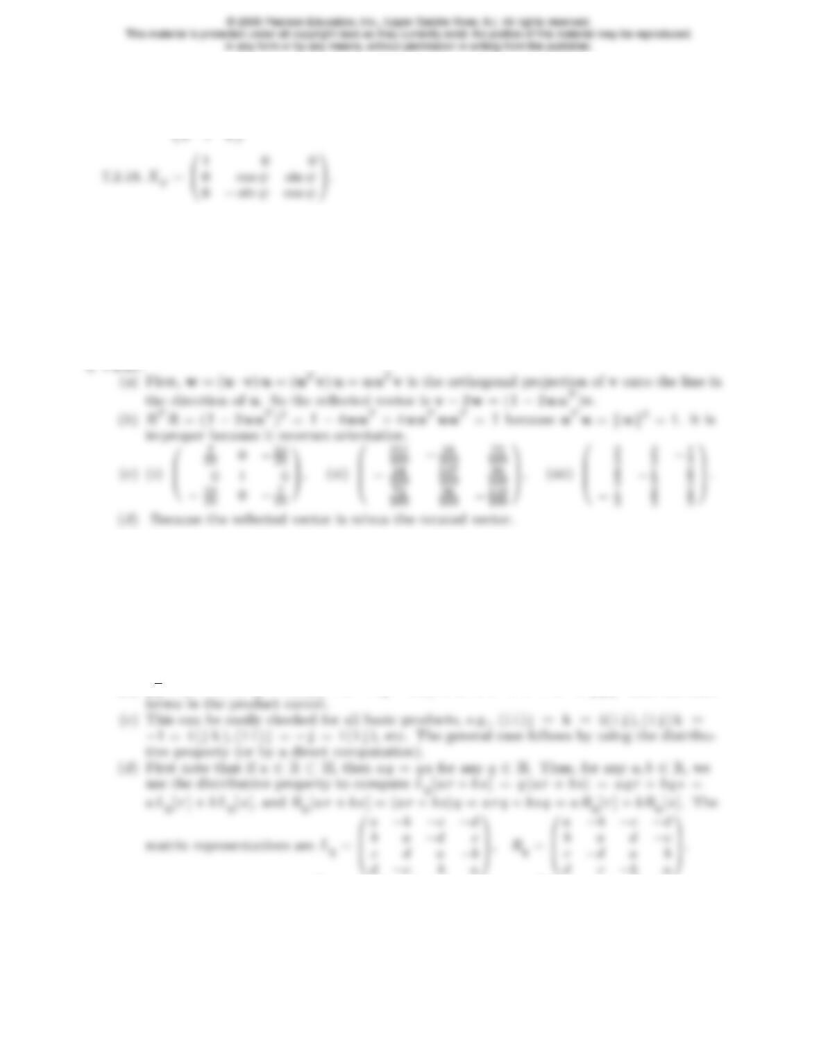
♦7.2.20. If vis orthogonal to u, then uTv= 0, and so Qπv=−v, while since kuk2=uTu= 1,
we have Qπu=u. Thus, uis fixed, while every vector in the plane orthogonal to it is ro-
tated through an angle π. This suffices to show that Qπrepresents the indicated rotation.
♦7.2.22. (a) In the formula for Rθ, the first factor rotates to align awith the zaxis, the sec-
ond rotates around the zaxis by angle θ, while the third factor QT=Q−1rotates the z
axis back to the line through a. The combined effect is a rotation through angle θaround
the axis a. (b) Set Q=0
B
@
1 0 0
0 0 −1
0 1 0 1
C
Aand multiply out to produce QZθQT=Yθ.
♥7.2.23.
(a) (i) 3 + i + 2 j , (ii ) 3 −i + j + k , (iii )−10 + 2 i −2 j −6 k , (iv ) 18.
(b)qq= (a+bi + cj + dk )(a−bi−cj−dk ) = a2+b2+c2+d2=kqk2since all other
(e) By direct computation: LT
qLq= (a2+b2+c2+d2) I = RT
qRq, and so LT
qLq= I =
RT
qRqwhen kqk2=a2+b2+c2+d2= 1.
(f) For q= ( b, c, d )T,r= ( x, y, z )T, we have q r = (bi + cj + dk )(xi + yj + zk ) =
188
For the exclusive use of adopters of the book Applied Linear Algebra, by Peter J. Olver and Cheri Shakiban. ISBN 0-13-147382-4.
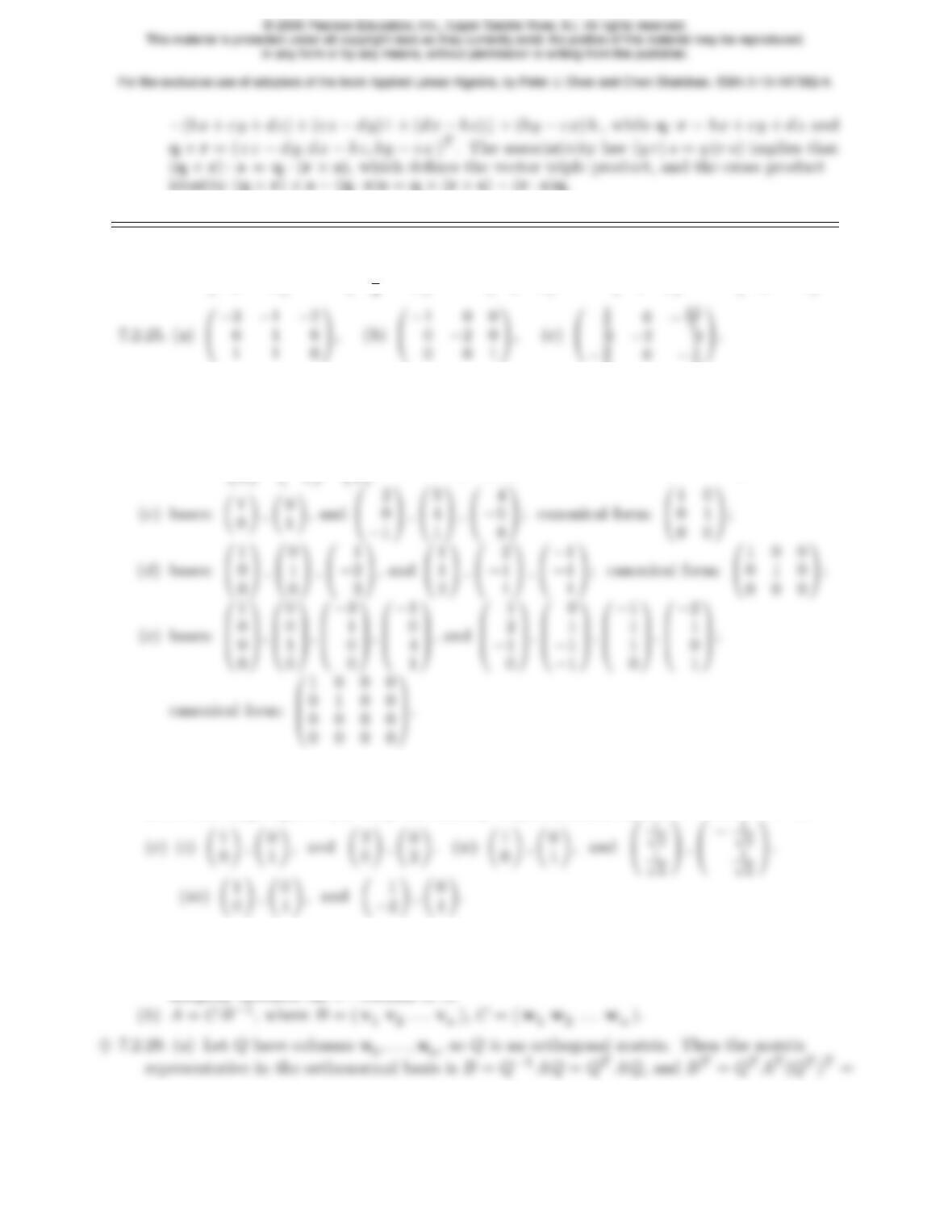
7.2.24. (a) 1−4
−2 3 !, (b) 1−6
−4
2 5 !, (d) −1 0
0 5 !, (e) −3−8
2 7 !.
50−1
5
7.2.26.
(a) Bases: 1
0!, 0
1!, and 1
2!, 2
1!; canonical form: 1 0
0 1 !;
(b) bases: 0
B
@
1
0
C
A,0
B
@−4
0
C
A,0
B
@
0
4
C
A, and 1
−2!, 2
1!; canonical form: 1 0 0
000!;
7.2.27. (a) Let v1,…,vnbe any basis for the domain space and choose wi=L[vi] for i=
1, . . . , n. Invertibility implies that w1,…,wnare linearly independent, and so form a ba-
sis for the target space. (b) Only the identity transformation, since A=SIS−1= I .
♦7.2.28.
(a) Given any v∈Rn, write v=c1v1+···+cnvn; then Av=c1Av1+···+cnAvn=
c1w1+··· +cnwn, and hence Avis uniquely defined. In particular, the value of Aei
189
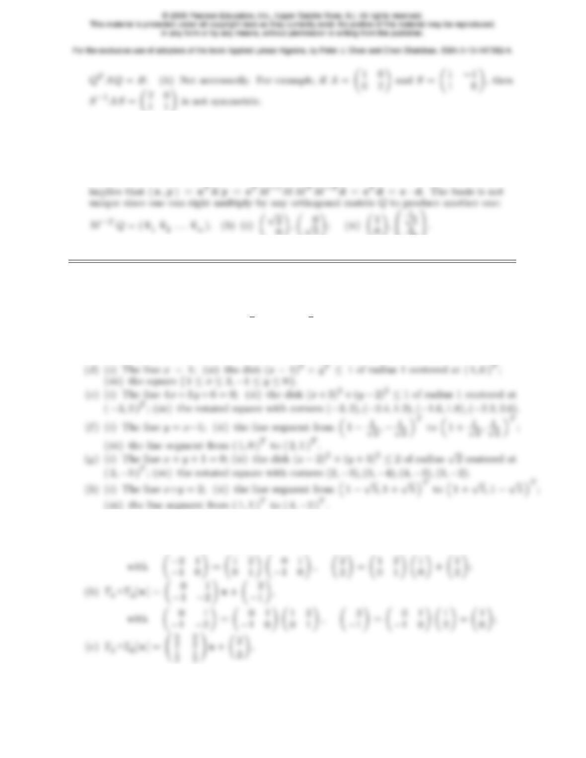
7.2.30. (a) Write hx,yi=xTKywhere K > 0. Using the Cholesky factorization (3.70), write
K=M MTwhere Mis invertible. Let M−T= ( v1v2. . . vn) define the basis. Then
x=
n
X
i= 1
civi=M−Tc,y=
n
X
i= 1
divi=M−Td,
7.3.1.
(a) (i) The horizontal line y=−1; (ii ) the disk (x−2)2+ (y+ 1)2≤1 of radius 1 centered
at ( 2,−1 )T; (iii ) the square {2≤x≤3,−1≤y≤0}.
(b) (i) The x-axis; (ii ) the ellipse 1
9(x+ 1)2+1
4y2≤1;
(iii ) the rectangle {−1≤x≤2,0≤y≤2}.
(c) (i) The horizontal line y= 2; (ii ) the elliptical domain x2−4xy+5y2+6 x−16 y+12 ≤0;
(iii ) the parallelogram with vertices ( 1,2 )T,( 2,2 )T,( 4,3 )T,( 3,3 )T.
7.3.2.
(a)T3◦T4[x] = −2 1
−1 0 !x+ 2
2!,
190