Solutions — Chapter 5
5.1.1. (a) Orthogonal basis; (b) orthonormal basis; (c) not a basis; (d) basis; (e) orthogonal
basis; (f) orthonormal basis.
5.1.2. (a) Basis; (b) orthonormal basis; (c) not a basis.
5.1.3. (a) Basis; (b) basis; (c) not a basis; (d) orthogonal basis; (e) orthonormal basis; (f) basis.
01
01
11
product, hv1,v2i=b > 0, since the coefficients of a, b, c appearing in the inner product
must be strictly positive.
♥5.1.10.
(a) By direct computation: u×v=u×w=0.
(b) First, if w=cv, then we compute v×w=0. Conversely, suppose v6=0— otherwise
the result is trivial, and, in particular, v16= 0. Then v×w=0implies wi=c vi,
♦5.1.11. See Example 5.20.
♦5.1.12. We repeatedly use the identity sin2α+ cos2α= 1 to simplify
hu1,u2i=−cos φsin φsin2θ+ (−cos θcos ψsin φ−cos φsin ψ)(cos θcos ψcos φ−sin φsin ψ)
+(cos ψsin φ+ cos θcos φsin ψ)(cos φcos ψ−cos θsin φsin ψ) = 0.
By similar computations, hu1,u3i=hu2,u3i= 0, hu1,u1i=hu2,u2i=hu3,u3i= 1.
120
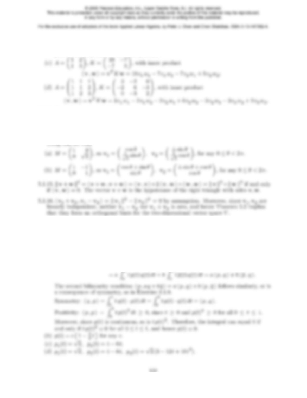
(b) According to part (a), orthonormality requires ATK A = I , and so K=A−TA−1=
(AAT)−1is the Gram matrix for A−1, and K > 0 since A−1is nonsingular. This also
proves the uniqueness of the inner product.
5.1.14. One way to solve this is by direct computation. A more sophisticated approach is to
apply the Cholesky factorization (3.70) to the inner product matrix: K=M M T. Then,
hv,wi=vTKw=b
vTb
wwhere b
v=Mv,b
w=Mw. Therefore, v1,v2form an orthonor-
mal basis relative to hv,wi=vTKwif and only if b
v1=Mv1,b
v2=Mv2,form an
orthonormal basis for the dot product, and hence of the form determined in Exercise 5.1.11.
Using this we find:
5.1.17. By orthogonality, the Gram matrix is a k×kdiagonal matrix whose diagonal entries
are kv1k2,…,kvkk2. Since these are all nonzero, the Gram matrix is nonsingular. An
alternative proof combines Propositions 3.30 and 5.4.
5.1.18.
(a) Bilinearity: for a, b constant,
ha p +be
p , q i=Z1
0t(a p(t) + be
p(t)) q(t)dt
5.1.19. Since Zπ
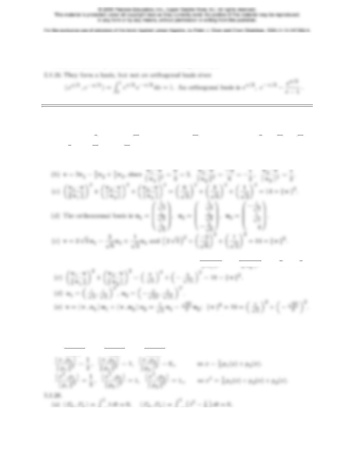
−πsin xcos x dx = 0, the functions cos xand sin xare orthogonal under the L2
inner product on [−π, π ]. Moreover, they span the solution space of the differential equa-
tion, and hence, by Theorem 5.5, form an orthogonal basis.
5.1.21.
(a) We compute hv1,v2i=hv1,v3i=hv2,v3i= 0 and kv1k=kv2k=kv3k= 1.
(b)hv,v1i=7
5,hv,v2i=11
13 , and hv,v3i=−37
65 , and so ( 1,1,1 )T=7
5v1+11
13 v2−37
65 v3.
(c)“7
5”2+“11
13 ”2+“−37
65 ”2= 3 = kvk2.
♥5.1.22.
(a) By direct commputation: v1·v2= 0, v1·v3= 0, v2·v3= 0.
5.1.23. (a) Because hv1,v2i=vT
1Kv2= 0. (b)v=hv,v1i
3v1−1
3v2.
5.1.24. Consider the non-orthogonal basis v1= 1
1!,v2= 0
1!. We have v= 1
0!=v1−v2,
but kvk2= 1 6= 12+ (−1)2.
5.1.25. h1, p1i
kp1k2= 1,h1, p2i
kp2k2= 0,h1, p3i
kp3k2= 0,, so 1 = p1(x) + 0 p2(x) + 0 p3(x) = p1(x).
−1t dt = 0, hP0, P2i=Z1
−1“t2−1
3”dt = 0,
122
hP0, P3i=Z1
−1“t3−3
5t”dt = 0, hP1, P2i=Z1
−1t“t2−1
3”dt = 0,
5.1.27.
(a)hP0, P1i=Z1
0“t−2
3”t dt = 0, hP0, P2i=Z1
0“t2−6
5t+3
10 ”t dt = 0,
5.1.29. 1
√2π,cos x
√π,sin x
√π, . . . , cos nx
√π,sin nx
√π.
♦5.1.30. heik x , e il x i=1
2πZπ
−πeik x eik x dx =1
2πZπ
−πei (k−l)xdx =(1, k =l,
0, k 6=l.
♦5.1.31.
Zπ
−πcos k x cos l x dx =Zπ
−π
1
2“cos(k−l)x+ cos(k+l)x”dx =8
>
>
>
<
>
>
>
:
0, k 6=l,
2π, k =l= 0,
π, k =l6= 0,
123
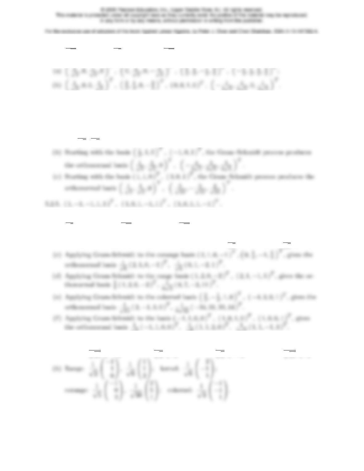
(c)1
√14 ( 1,2,3 )T,1
√3( 1,1,−1 )T,1
√42 (−5,4,−1 )T.
5.2.2.
5.2.3. The first two Gram–Schmidt vectors are legitimate, v1= ( 1,−1,0,1 )T,v2= ( −1,0,1,1 )T,
but then v3=0, and the algorithm breaks down. The reason is that the given vectors are
linearly dependent, and do not, in fact, form a basis.
5.2.4.
(a) 0,2
√5,1
√5!T
,( 1,0,0 )T.
5.2.6.
(a)1
√3( 1,1,−1,0 )T,1
√15 (−1,2,1,3 )T,1
√15 ( 3,−1,2,1 )T.
(b) Solving the homogeneous system we obtain the kernel basis ( −1,2,1,0 )T, ( 1,−1,0,1 )T.
The Gram-Schmidt process gives the orthonormal basis 1
√6(−1,2,1,0 )T,1
√6( 1,0,1,2 )T.
2√3( 1,1,−1,3 )T.
5.2.7.
(a) Range: 1
√10 1
−3!; kernel: 1
√2 1
1!; corange: 1
√2 1
−1!; cokernel: 1
√10 3
1!.
124
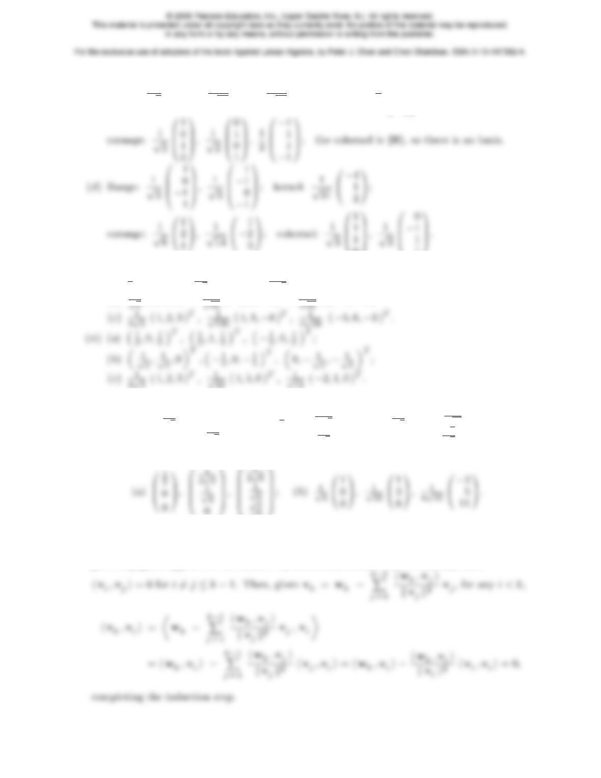
(c) Range: 1
√30
B
@
1
1
−11
C
A,1
√42 0
B
@
1
4
51
C
A,1
√14 0
B
@
3
−2
11
C
A; kernel: 1
20
B
B
B
@
−1
−1
1
1
1
C
C
C
A;
0
1
5.2.8.
(i) (a)1
2( 1,0,1 )T,1
√2( 0,1,0 )T,1
2√3(−1,0,3 )T;
(b)1
√5( 1,1,0 )T,1
√55 (−2,3,−5 )T,1
√66 ( 2,−3,−6 )T;
5.2.9. Applying the Gram–Schmidt process to the standard basis vectors e1,e2gives
(a)0
@
1
√3
01
A,0
@0
1
√51
A; (b)0
@
1
2
01
A,0
B
@
1
2√3
2
√3
1
C
A; (c)0
@
1
√2
01
A,0
B
@−1
√10
√2
√5
1
C
A.
5.2.10. Applying the Gram–Schmidt process to the standard basis vectors e1,e2,e3gives
1
1
5.2.11. (a) 2, namely ±1; (b) infinitely many; (c) no.
♦5.2.12. The key is to make sure the inner products are in the correct order, as otherwise com-
plex conjugates appear on the scalars. By induction, assume that we already know
125
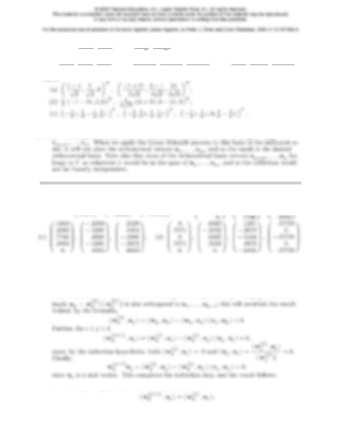
5.2.13. (a) 1 + i
2,1−i
2!T
, 3−i
2√5,1 + 3 i
2√5!T
;
(b) 1 + i
3,1−i
3,2−i
3!T
, −2 + 9 i
15 ,−9−7 i
15 ,−1 + 3 i
15 !T
, 3−i
5,1−2 i
5,−1 + 3 i
5!T
.
5.2.15. False. Any example that starts with a non-orthogonal basis will confirm this.
♦5.2.16. According to Exercise 2.4.24, we can find a basis of Rnof the form u1, . . . , um,
5.2.17. (a)0
B
@
0.
.7071
C
A,0
B
@
.8165
−.4082
C
A,0
B
@
.57735
.57735
C
A; (b)0
B
B
B
@
.57735
.57735
−.57735
1
C
C
C
A,0
B
B
B
@
−.2582
.5164
.2582
1
C
C
C
A,0
B
B
B
@
.7746
−.2582
.5164
1
C
C
C
A;
5.2.18. Same solutions.
5.2.19. See previous solutions.
♦5.2.20. Clearly, each uj=w(j)
j/kw(j)
jkis a unit vector. We show by induction on kand then
on jthat, for each 2 ≤j≤k, the vector w(j)
5.2.21. Since u1, . . . , unform an orthonormal basis, if i < j,
126
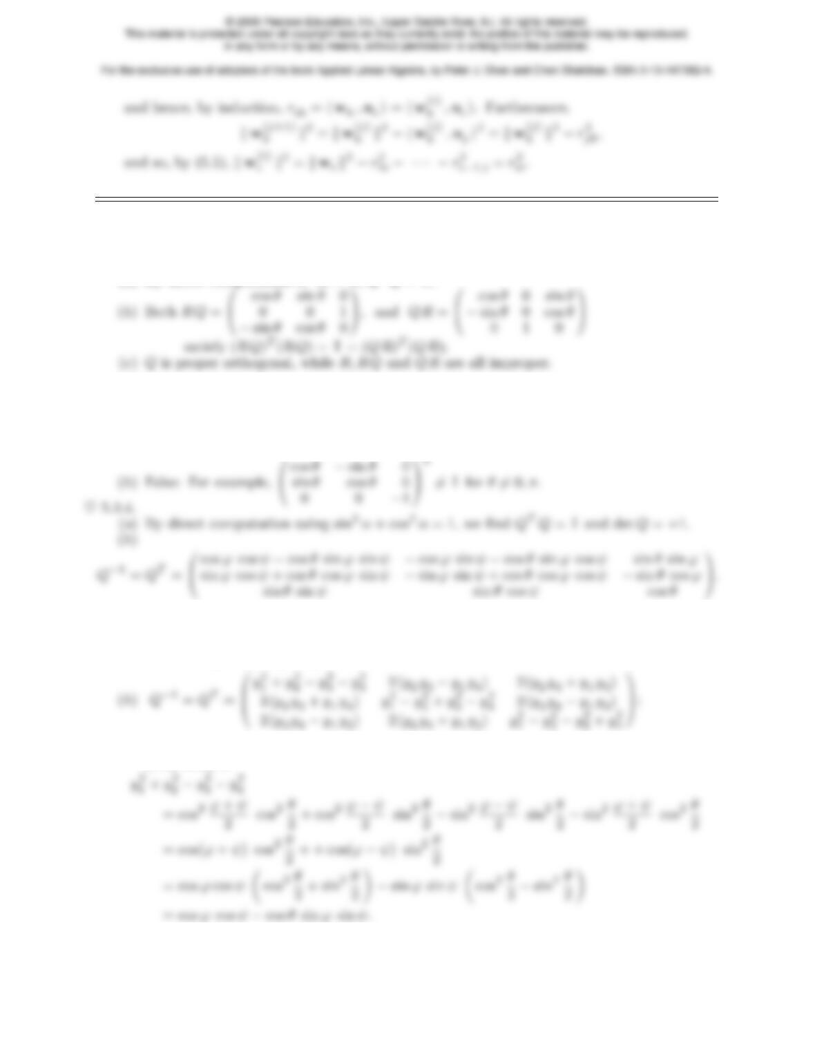
5.3.1. (a) Neither; (b) proper orthogonal; (c) orthogonal; (d) proper orthogonal; (e) neither;
(f) proper orthogonal; (g) orthogonal.
5.3.2.
(a) By direct computation RTR= I , QTQ= I ;
5.3.3.
(a) True: Using the formula (5.31) for an improper 2 ×2 orthogonal matrix,
cos θsin θ
sin θ−cos θ!2
= 1 0
0 1 !.
♥5.3.5.
(a) By a long direct computation, we find QTQ= (y2
1+y2
2+y2
3+y2
4)2I and
det Q= (y2
1+y2
2+y2
3+y2
4)3= 1.
(c) These follow by direct computation using standard trigonometric identities, e.g., the
(1,1) entry is
5.3.6. Since the rows of Qare orthonormal (see Exercise 5.3.8), so are the rows of Rand hence
127
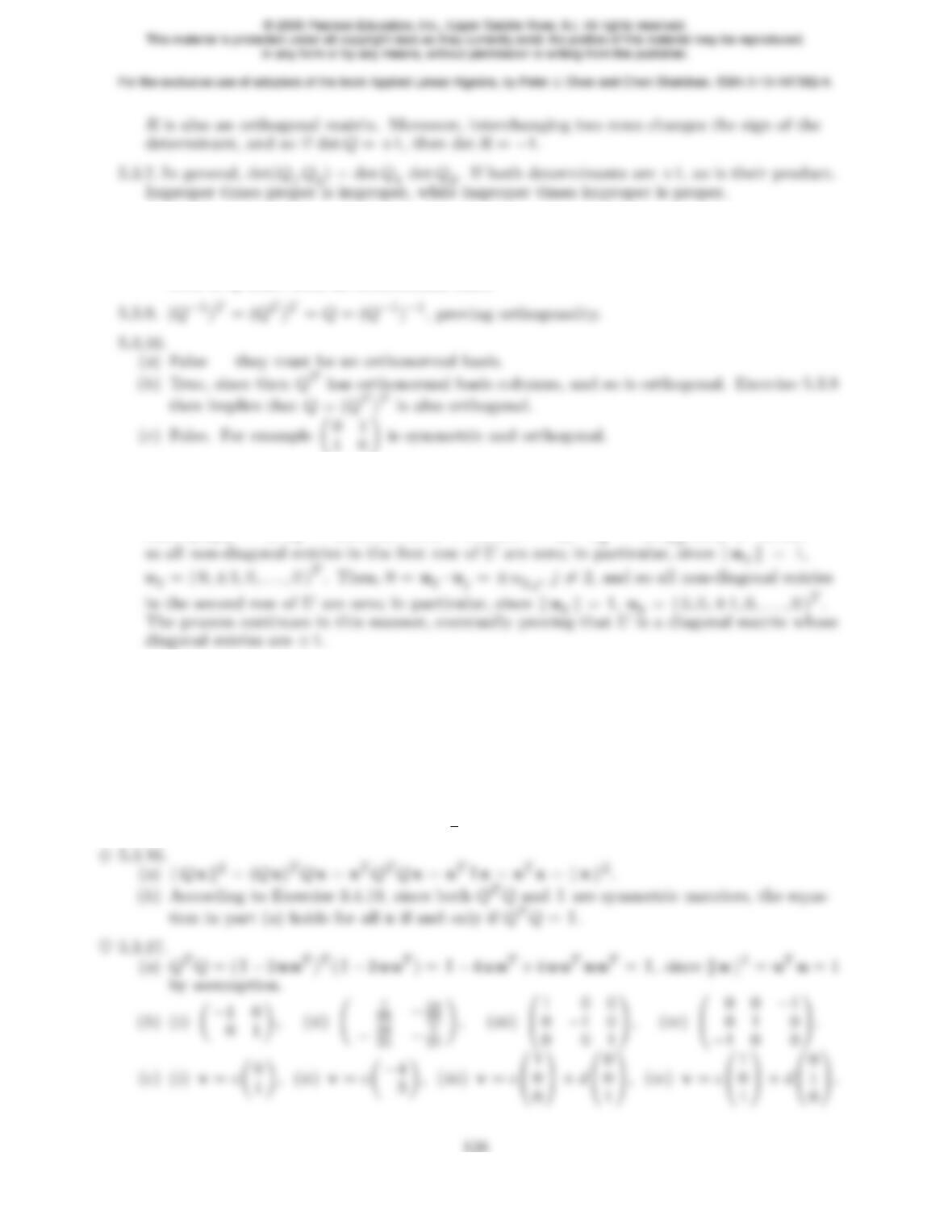
♦5.3.8.
(a) Use (5.30) to show (QT)−1=Q= (QT)T.
(b) The rows of Qare the columns of QT, and hence since QTis an orthogonal matrix, the
rows of Qmust form an orthonormal basis.
5.3.11. All diagonal matrices whose diagonal entries are ±1.
5.3.12. Let U= ( u1u2. . . un), where the last n−jentries of the jth column ujare zero.
Since ku1k= 1, u1= ( ±1,0,…,0 )T. Next, 0 = u1·uj=±u1,j for j6= 1, and
5.3.13. (a) Note that P2= I and P=PT, proving orthogonality. Moreover, det P=−1
since Pcan be obtained from the identity matrix I by interchanging two rows. (b) Only
the matrices corresponding to multiplying a row by −1.
5.3.14. False. This is true only for row interchanges or multiplication of a row by −1.
5.3.15.
(a) The columns of Pare the standard basis vectors e1,…,en, rewritten in a different or-
der, which doesn’t affect their orthonormality.
(b) Exactly half are proper, so there are 1
2n! proper permutation matrices.
5.3.19.
(a) If S= ( v1v2… vn), then S−1=STD, where D= diag (1/kv1k2, . . . , 1/kvnk2).
1
1
0
1
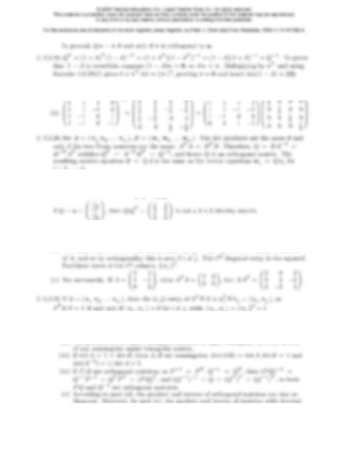
5.3.21. (a) The (i, j) entry of QTQis the product of the ith row of QTtimes the jth column of
Q, namely uT
iuj=ui·uj=(1, i =j,
5.3.22.
(a) Assuming the columns are nonzero, Proposition 5.4 implies they are linearly indepen-
dent. But there can be at most mlinearly independent vectors in Rm, so n≤m.
(b) The (i, j) entry of ATAis the dot product vT
♥5.3.24.
(a) Given any A∈G, we have A−1∈G, and hence the product AA−1= I ∈Galso.
(b) (i) If A, B are nonsingular, so are AB and A−1, with (AB)−1=B−1A−1, (A−1)−1=A.
(ii ) The product of two upper triangular matrices is upper triangular, as is the inverse
129
nant 1 also have determinant 1. Therefore, the product and inverse of proper or-
thogonal matrices are proper orthogonal.
(vi ) The inverse of a permutation matrix is a permutation matrix, as is the product of
two permutation matrices.
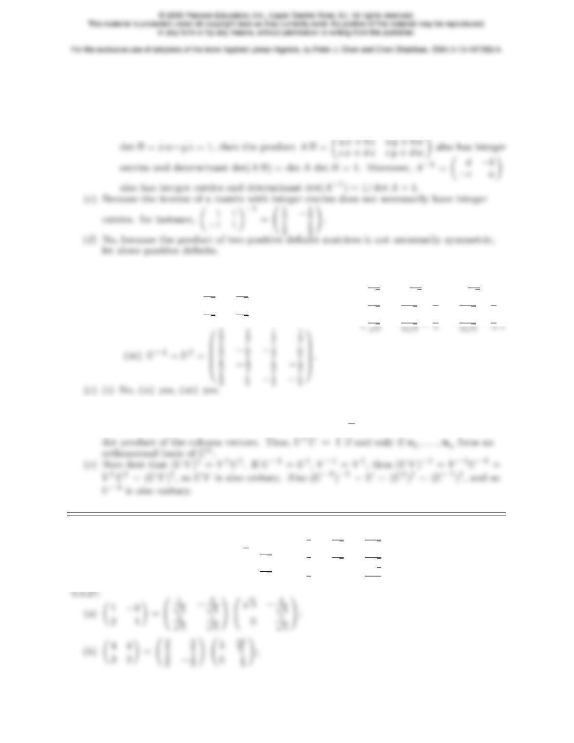
(vii ) If A= a b
c d !, B = x y
z w !have integer entries with det A=a d −bd = 1,
♥5.3.25.
(a) The defining equation U†U= I implies U−1=U†.
(b) (i)U−1=U†=0
B
@
1
√2−i
√2
−i
√2
1
√2
1
C
A, (ii )U−1=U†=0
B
B
B
B
@
1
√3
1
√3
1
√3
1
√3−1
2√3−i
2−1
2√3+i
2
1
√3−1
1
C
C
C
C
A,
(d) Let u1,…,undenote the columns of U. The ith row of U†is the complex conjugate of
the ith column of U, and so the (i, j) entry of U†Uis uT
iuj=uj·ui, i.e., the Hermitian
5.3.26. 0
B
B
@
2 0 1
2 4 2
−1−1−3
1
C
C
A=0
B
B
B
B
@
3 3 3
0 2√21
√2
0 0 3
√2
1
C
C
C
C
A
0
B
B
B
B
@
2
3−1
√2−1
3√2
2
31
√2−1
3√2
−1
30−2√2
3
1
C
C
C
C
A.
130
(c)0
B
B
@
2 1 −1
0 1 3
−1−1 1
1
C
C
A=0
B
B
B
B
B
@
2
√5−1
√30
1
√6
0q5
61
√6
−1
√5−q2
15 q2
3
1
C
C
C
C
C
A
0
B
B
B
B
@
√53
√5−3
√5
0q6
57q2
15
0 0 2q2
3
1
C
C
C
C
A;
(d)0
B
B
@
0 1 2
−111
−1 1 3
1
C
C
A=0
B
B
B
B
@
0 1 0
−1
√20−1
√2
−1
√201
√2
1
C
C
C
C
A0
B
B
@
√2−√2−2√2
0 1 2
0 0 √2
1
C
C
A;
2−1
2√3−1
5.3.28.
(i) (a) 1 2
−1 3 !=0
B
@
1
√2
1
√2
−1
√2
1
√2
1
C
A0
B
@
√2−1
√2
05
√2
1
C
A; (b) x
y!=0
@−7
5
1
51
A;
31
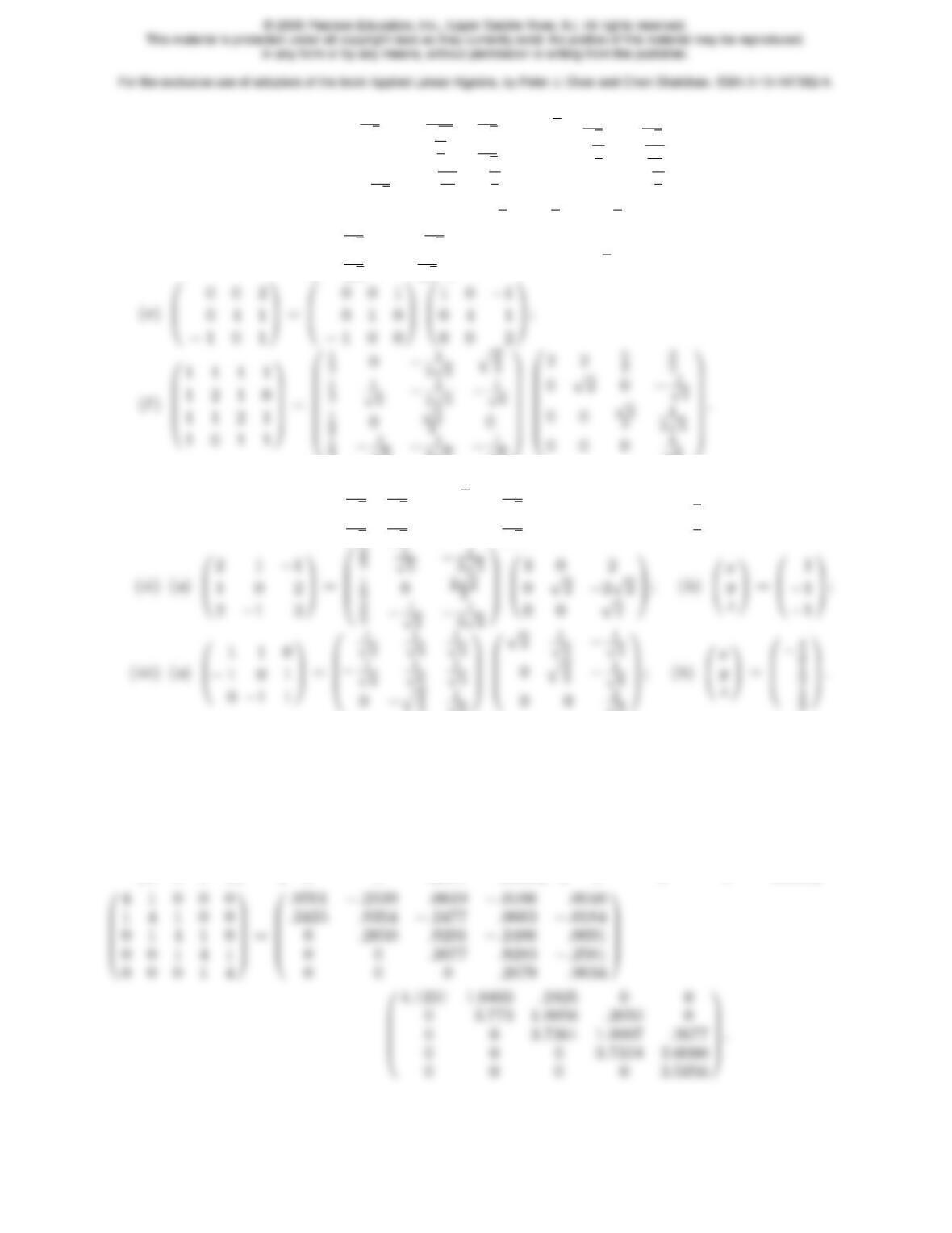
♠5.3.29.
0
B
@
4 1 0
1 4 1
0 1 4 1
C
A=0
B
@
.9701 −.2339 .0643
.2425 .9354 −.2571
0.2650 .9642 1
C
A0
B
@
4.1231 1.9403 .2425
0 3.773 1.9956
0 0 3.5998 1
C
A,
0
B
B
B
@
4 1 0 0
1 4 1 0
0 1 4 1
0 0 1 4
1
C
C
C
A=0
B
B
B
@
.9701 −.2339 .0619 −.0172
.2425 .9354 −.2477 .0688
0.2650 .9291 −.2581
0 0 .2677 .9635
1
C
C
C
A0
B
B
B
@
4.1231 1.9403 .2425 0
0 3.773 1.9956 .2650
0 0 3.7361 1.9997
0 0 0 3.596
1
C
C
C
A,
131
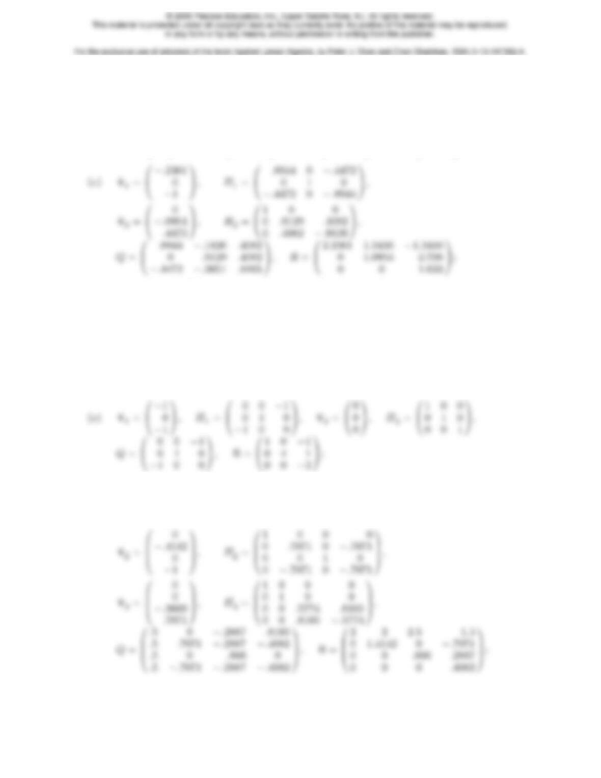
5.3.30. : 5.3.27 (a)b
v1= −1.2361
2.0000 !, H1= .4472 .8944
.8944 −.4472 !,
Q= .4472 .8944
.8944 −.4472 !, R = 2.2361 −.4472
0−3.1305 !;
(b)b
v1= −1
3!, H1= .8.6
.6−.8!, Q = .8.6
.6−.8!, R = 5 3.6
0.2!;
(d)b
v1=0
B
@−1.4142
−1
−11
C
A, H1=0
B
@
0−.7071 −.7071
−.7071 .5−.5
−.7071 −.5.51
C
A,
b
v2=0
B
@
0
−1.7071
−.7071 1
C
A, H2=0
B
@
1 0 0
0−.7071 −.7071
0−.7071 .7071 1
C
A
Q=0
B
@
0 1 0
−.7071 0 −.7071
−.7071 0 .7071 1
C
A, R =0
B
@
1.4142 −1.4142 −2.8284
0 1 2
0 0 1.4142 1
C
A;
(f)b
v1=0
B
B
B
@
−1
1
1
1
1
C
C
C
A, H1=0
B
B
B
@
.5.5.5.5
.5.5−.5−.5
.5−.5.5−.5
.5−.5−.5.5
1
C
C
C
A,
132
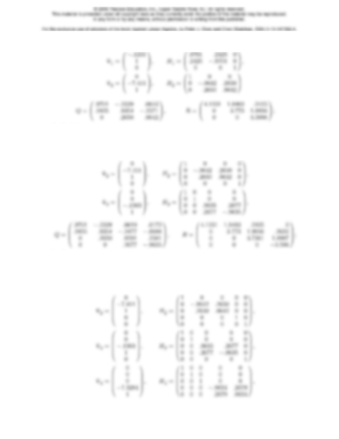
5.3.29: 3 ×3 case:
4×4 case:
b
v1=0
B
B
B
@
−.1231
1
0
0
1
C
C
C
A, H1=0
B
B
B
@
.9701 .2425 0 0
.2425 −.9701 0 0
0 0 1 0
0 0 0 1
1
C
C
C
A,
5×5 case:
b
v1=0
B
B
B
B
B
@
−.1231
1
0
0
0
1
C
C
C
C
C
A
, H1=0
B
B
B
B
B
@
.9701 .2425 0 0 0
.2425 −.9701 0 0 0
0 0 1 0 0
0 0 0 1 0
0 0 0 0 1
1
C
C
C
C
C
A
,
133
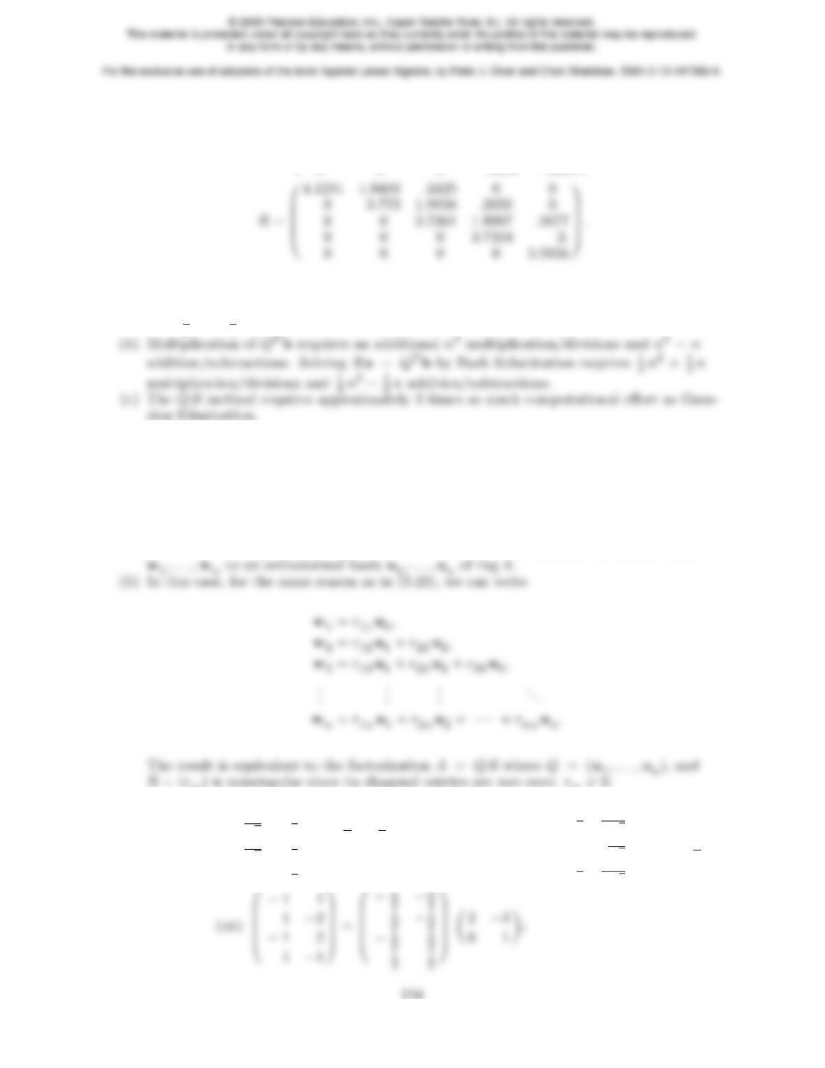
Q=0
B
B
B
B
B
@
.9701 −.2339 .0619 −.0166 .0046
.2425 .9354 −.2477 .0663 −.0184
0.2650 .9291 −.2486 .0691
0 0 .2677 .9283 −.2581
000.2679 .9634
1
C
C
C
C
C
A
,
♥5.3.31.
(a)QR factorization requires n3+n2multiplication/divisions, nsquare roots, and
n3−1
2n2−1
2naddition/subtractions.
♦5.3.32. If QR =e
Qe
R, then Q−1e
Q=e
R R−1. The left hand side is orthogonal, while the
right hand side is upper triangular. Thus, by Exercise 5.3.12, both sides must be diagonal
with ±1 on the diagonal. Positivity of the entries of Rand e
Rimplies positivity of those of
e
R R−1, and hence Q−1e
Q=e
R R−1= I , which implies Q=e
Qand R=e
R.
♥5.3.33.
(a) If rank A=n, then the columns w1,…,wnof Aare linearly independent, and so form
a basis for its range. Applying the Gram–Schmidt process converts the column basis
(c)
(i)0
B
B
@
1−1
2 3
0 2
1
C
C
A=0
B
B
B
B
@
1
√5−2
3
2
√5
1
3
02
3
1
C
C
C
C
A √5√5
0 3 !; (ii )0
B
B
@−3 1
0 1
4 2
1
C
C
A=0
B
B
B
B
@
−3
58
5√5
01
√5
4
56
5√5
1
C
C
C
C
A 5 1
0√5!;
1
1
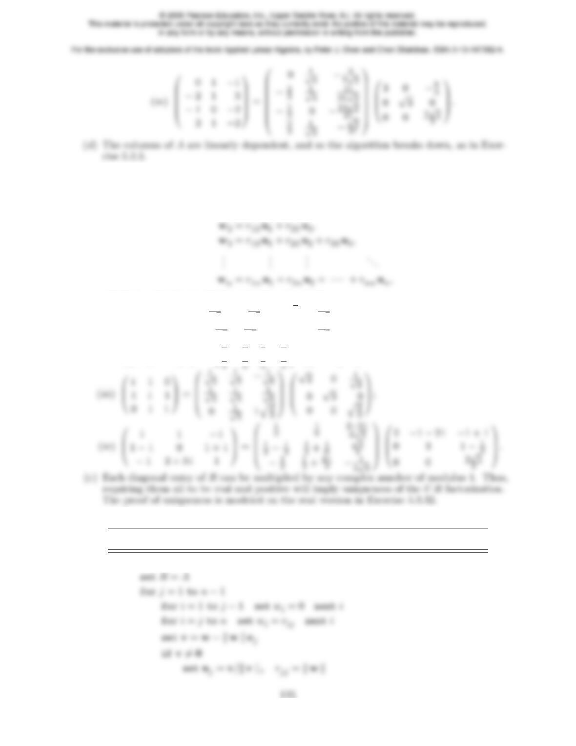
♥5.3.34.
(a) If A= ( w1w2. . . wn), then U= ( u1u2. . . un) has orthonormal columns and hence
is a unitary matrix. The Gram-Schmidt process takes the same form:
w1=r11 u1,
which is equivalent to the factorization A=U R.
(b) (i) i 1
−1 2 i !=0
B
@
i
√2−1
√2
−1
√2
i
√2
1
C
A0
B
@
√2−3 i
√2
01
√2
1
C
A;
(ii ) 1 + i 2 −i
1−i−i!=0
@
1
2+i
21
2−i
2
1
A 2 1 −2 i
0 1 !;
5.3.35.
Householder’s Method
start
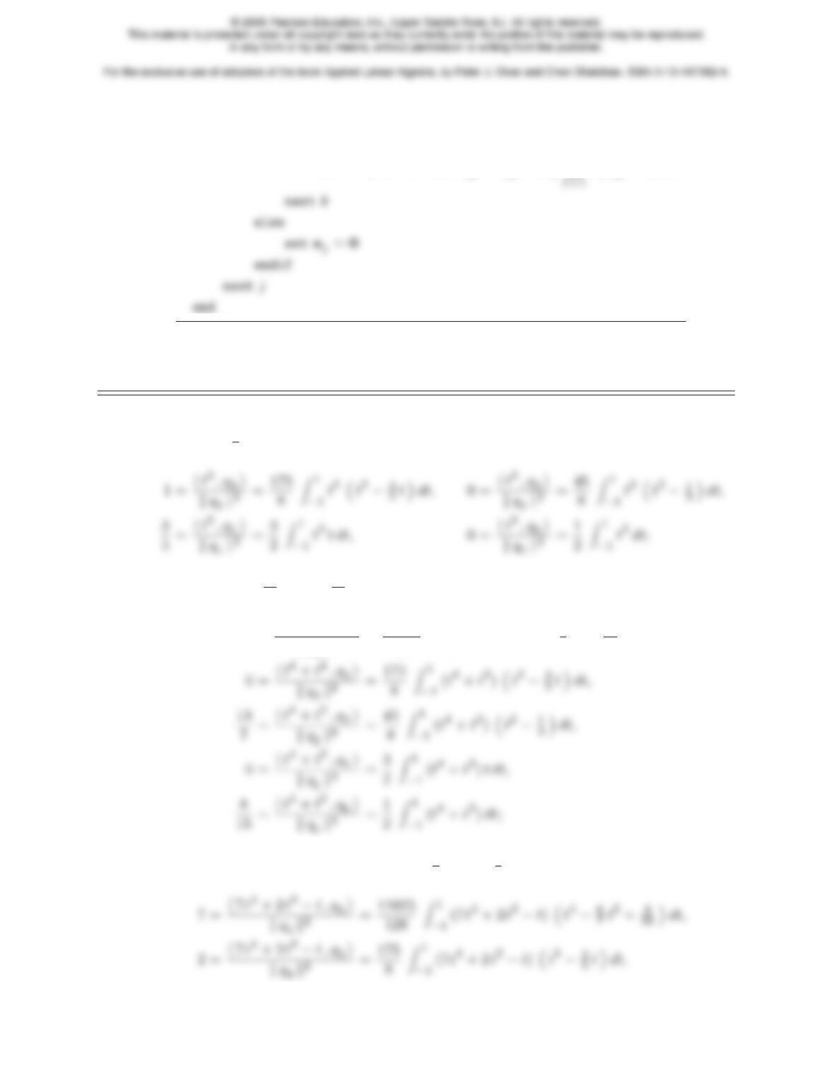
for i=j+ 1 to nset rij = 0 next i
for k=j+ 1 to n
for i=jto nset rik =rik −2ui
n
X
ulrlk next i
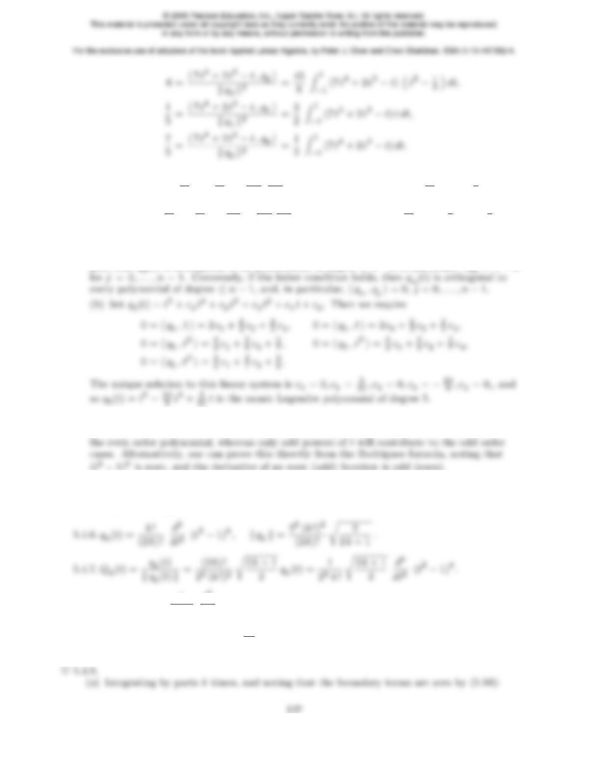
5.4.1.
(a)t3=q3(t) + 3
5q1(t), where
(b)t4+t2=q4(t) + 13
7q2(t) + 8
15 q0(t), where
1 = ht4+t2, q4i
kq4k2=11025
128 Z1
−1(t4+t2)“t4−6
7t2+3
35 ”dt,
(c) 7t4+ 2t3−t= 7q4(t) + 2q3(t) + 6q2(t) + 1
5q1(t) + 7
5q0(t), where
136
5.4.2. (a)q5(t) = t5−10
9t3+5
21 t=5!
10!
d5
dt5(t2−1)5, (b)t5=q5(t) + 10
9q3(t) + 3
7q1(t),
(c)q6(t) = t6−15
11 t4+5
11 t2−5
231 =6!
12!
d6
dt6(t2−1)6,t6=q6(t)+ 15
11 q4(t)+ 5
7q2(t)+ 1
7q0(t).
♦5.4.3. (a) We characterized qn(t) as the unique monic polynomial of degree nthat is orthogo-
nal to q0(t),…,qn−1(t). Since these Legendre polynomials form a basis of P(n−1), this im-
plies that qn(t) is orthogonal to all polynomials of degree ≤n−1; in particular hqn, tji= 0
5.4.4. Since even and odd powers of tare orthogonal with respect to the L2inner product on
[−1,1], when the Gram–Schmidt process is run, only even powers of twill contribute to
5.4.5. Use Exercise 5.4.4 and the fact that hf , g i=Z1
−1f(t)g(t)dt = 0 if fis odd and gis
even, since their product is odd.
♦5.4.8. Write Pk(t) = 1
2kk!
dk
dtk(t−1)k(t+ 1)k.Differentiating using Leibniz’ Rule, we con-
clude the only term that does not contain a factor of t−1 is when all kderivatives are ap-
plied to (t−1)k. Thus, Pk(t) = 1
2k(t+ 1)k+ (t−1) Sk(t) for some polynomial Sk(t) and so
Pk(1) = 1.
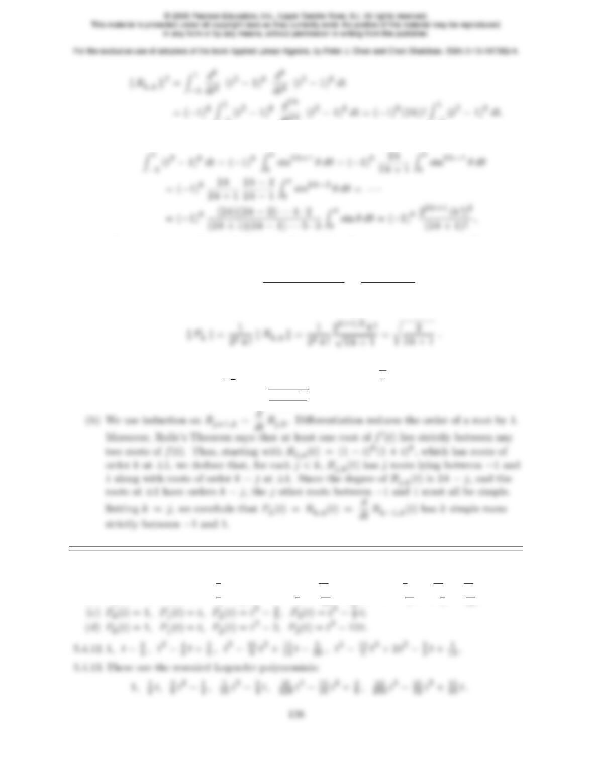
−1(t2−1)kd2k
dt2k(t2−1)kdt = (−1)k(2k)! Z1
−1(t2−1)kdt.
(b) Since t= cos θsatisfies dt =−sin θ dθ, and takes θ= 0 to t= 1 and θ=πto t=−1, we
find
where we integrated by parts ktimes after making the trigonometric change of vari-
ables. Combining parts (a,b),
kRk,k k2=(2 k) ! 22k+1 (k!)2
(2k+ 1)! =22k+1 (k!)2
2k+ 1 .
Thus, by the Rodrigues formula,
♥5.4.10.
(a) The roots of P2(t) are ±1
√3; the roots of P3(t) are 0,±q3
5;
the roots of P4(t) are ±r15±2√30
35 .
5.4.11.
(a)P0(t) = 1, P1(t) = t−3
2, P2(t) = t2−3t+13
6, P3(t) = t3−9
2t2+33
5t−63
20 ;
(b)P0(t) = 1, P1(t) = t−2
3, P2(t) = t2−6
5t+3
10 , P3(t) = t3−12
7t2+6
7t−4
35 ;
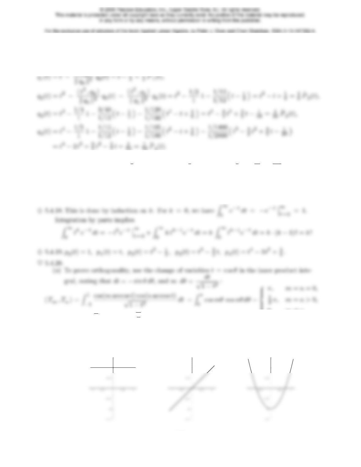
5.4.14. Setting hf , g i=Z1
0f(t)g(t)dt,kfk2=Z1
0f(t)2dt,
q0(t) = 1 = e
P0(t),
5.4.15. p0(t) = 1, p1(t) = t−1
2, p2(t) = t2−t+1
6, p3(t) = t3−3
2t2+33
65 t−1
260 .
♦5.4.16. The formula for the norm follows from combining equations (5.48) and (5.59).
5.4.17. L4(t) = t4−16t3+ 72 t2−96t+ 24,kL4k= 24,
L5(t) = t5−25t4+ 200t3−600t2+ 600t−120,kL5k= 120.
0, m 6=n.
(b)kT0k=√π , kTnk=qπ
2,for n > 0.
(c)T0(t) = 1, T1(t) = t, T2(t) = 2t2−1, T3(t) = 4t3−3t,
T4(t) = 8t4−8t2+ 1, T5(t) = 16t5−20t3+ 5t, T6(t) = 32 t6−48 t4+ 18 t2−1.
1
1.5
1
1.5
1
1.5
139