Chapter 5
5.2
2
0
(1 ) 1
lim 2
(1)
tktkttkt
t
t
e e ke ke k
ek
μ
5.3
(0) 1f
θ
,
(1)f
θ
μ
5.4
μ
θ
2
μ
θ
22
(1 )
σθθθ θ
μ
μ
μ
5.5 (a)
()
(; , 1) (1)
(1 ) ( ; , )
nx n nx
xnx
n
bn x n nx
nbx n
x
θθθ
θθ θ
62 Mathematical Statistics, 8E
5.6 (a)
1
11
( ; , ) ( 1; , ) ( ; , )
xx
ii
Bx n Bx n bxn
θθ θ
(b)
()
( ; , 1 ) ( 1; , 1 )
( ; , 1 ) (1 )
= (1 ) ( ; , )
nx n nx
xnx
Bn xn Bn x n
n
bn x n nx
nbx n
x
θθ
θθθ
θθ θ
5.7
1
() ( )
Xn
EY E E X
nn n
θθ
2
22
222
1[(1 )
X
Enn
nn
μ
θθ θ
2 2 22 22
2
1(1)
[]
Y
nn n n n
n
θθ
σθθθθ
Chapter 5 63
2
2
5.10
(; , ) (1 )
xnx
n
bx n x
θθθ
ln ln ln ( )ln(1 )
n
bxnx
x
θθ
0
1
bxnx
θθ θ
xxn x
θθθ
xn
θ
and
x
n
θ
5.12
1
() ()
x
Fx xt fx
1
(1) ( ) ( )Fxfx
μ
2
() ( 1) ()
x
Fx xx t fx
2
(1) ( 1) ( ) ( )Fxxfx
μ
3
() ( 1)( 2) ()
x
Fx xx x tfx
3
(1) ( 1)( 2) ( ) ( )Fxxxfx
μ
etc.
(1)
()
r
64 Mathematical Statistics, 8E
5.14
() ()( ) [ () ()]
ttt
YXX XX
M eMt Mt e e Mt Mt
μμμ
μμ
(a) Expand series.
(b)
() [1 ( 1)]
nt t n
X
Mte e
θ
μ
θ
1
() [1 ( 1) [1 ( 1)]
nt t n t nt t n
x
Mte n e ene e
θθ
μ
θθθθ
5.15 (a)
3
1, 0;
2
θα
(b)
3
0 as n
α
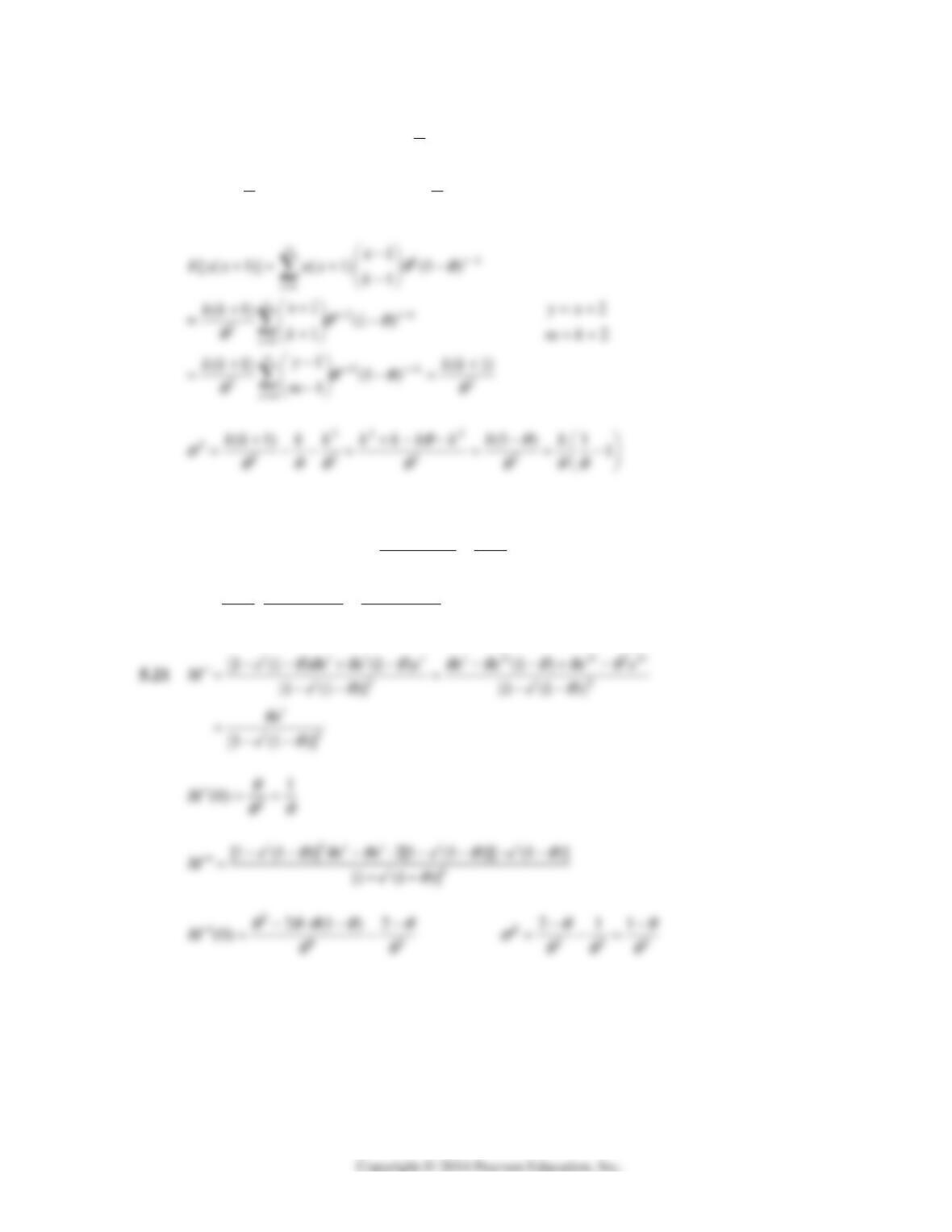
5.16
1
() (1 )
1
ky
yk
fy k
θθ
0, 1, 2,
yxk
y
Chapter 5 65
5.19
1
1
() (1 ) (1 )
1
kxk x xk
xk xk
xx
k
Ex x kk
θθ θ θ
θ
1
1
yx
mk
=
1(1 )
1
yym
ym
y
kk
m
θθ
θθ
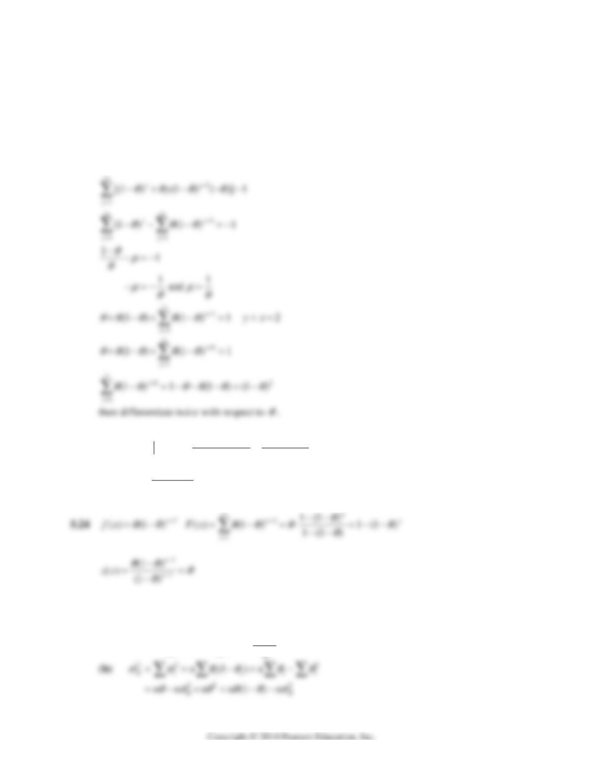
5.20
1
() (1 )
x
gx
θθ
1, 2, 3,x
1
11 1
[(1 )]
(1 ) [ (1 )]
11
(1 ) QED
11(1)1(1)
tx
tx x t x
xx x
tt
tt
e
Me e
ee
ee
θθ
θθ θ θ
θθ
θθθ
θθθ
66 Mathematical Statistics, 8E
5.22
1
1
(1 ) 1
x
x
θθ
1
2
(1 ) 1
x
x
θθθ
1yx
1
(1 ) 1
y
y
θθ θ
5.23
()(1)
() (1)
()(1 )
xn
x
n
PX x n
PX x nx n PX n
θθ θθ
θ
QED
(1 )
() (1)
1(1 )
n
n
PX n
θθ θ
θ
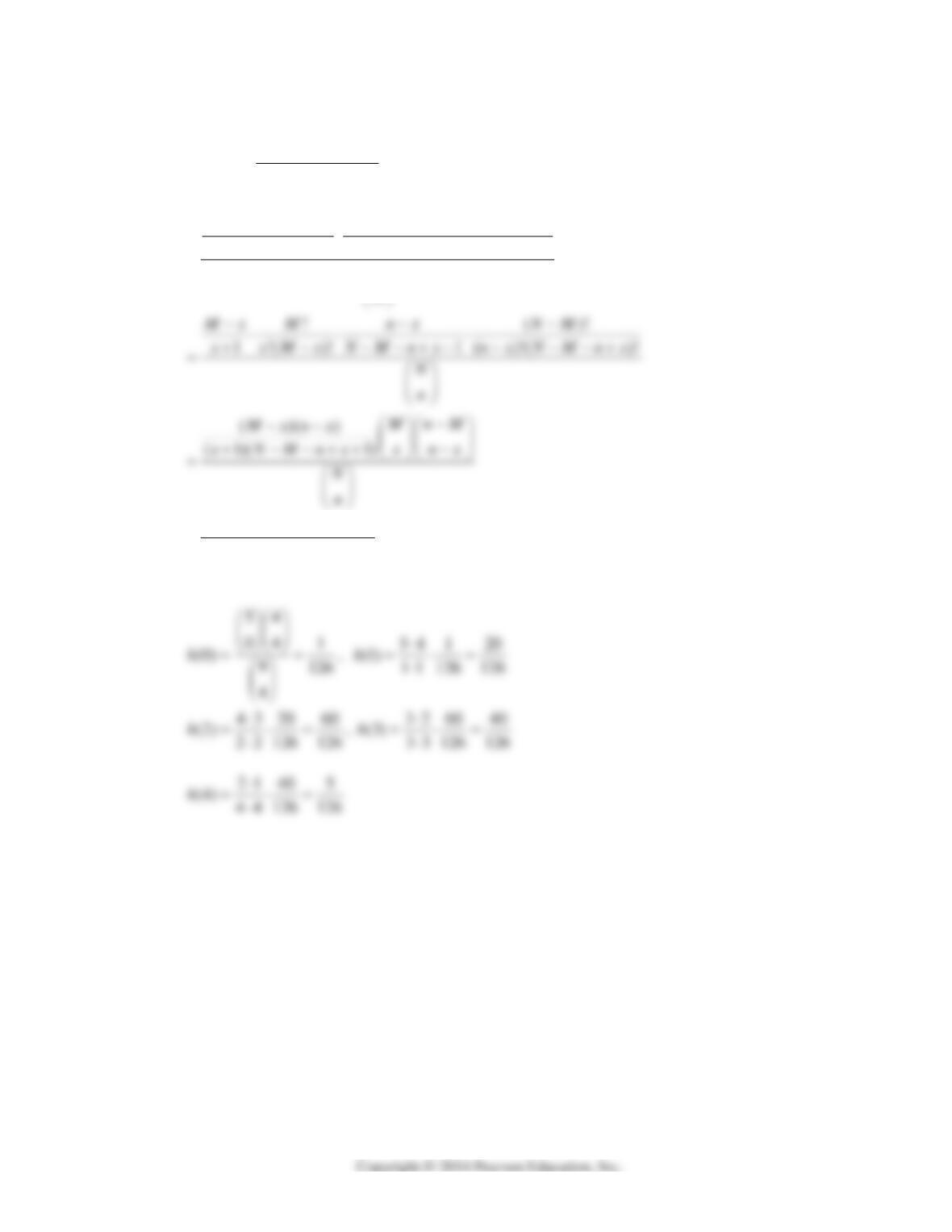
5.25
12 n
XX X X
(a)
() ( )
i
ii
EX EX n n
θ
θθ
Chapter 5 67
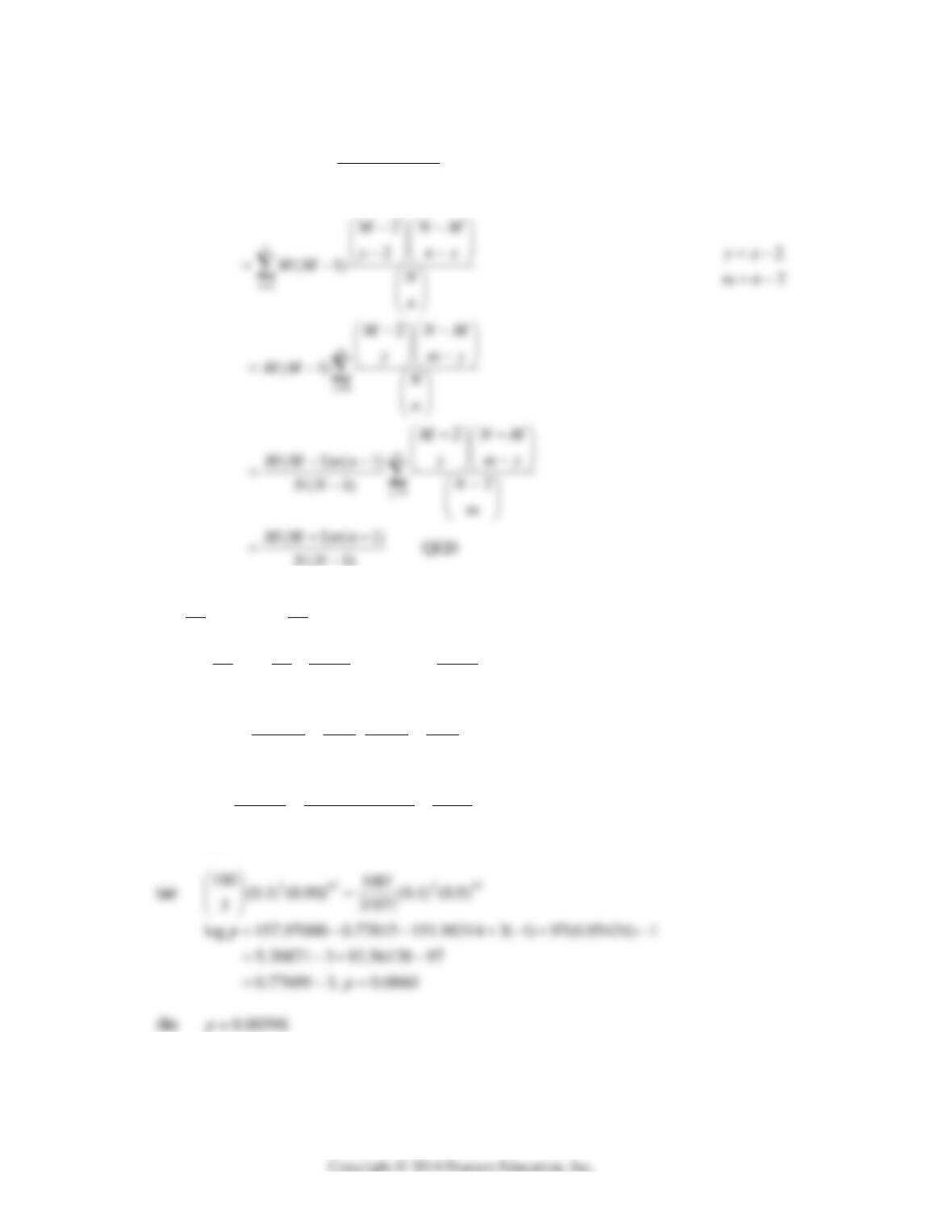
5.26
11
(1)
MnM
xnx
hx N
n
!()!
( 1)!( 1)! ( 1)!( 1)!
()() (
(1)( 1)
MNM
xMx nxNMnx
N
n
Mxnx hx
xNMnx
)
4, 9, 5nNM
68 Mathematical Statistics, 8E
5.27
0
[( 1)] ( 1)
n
x
MNM
nx
x
EX X xx N
n
(1)
NN
5.28
M
N
θ
M
nn
N
μ
θ
2
1(1)
11
M M Nn Nn
nn
NNN N
σθθ
5.29
1
( 1; ) ( ; )
(1)! 1 ! 1
xx
ee
Px px
xxxx
λλ
λλλλ
λλ
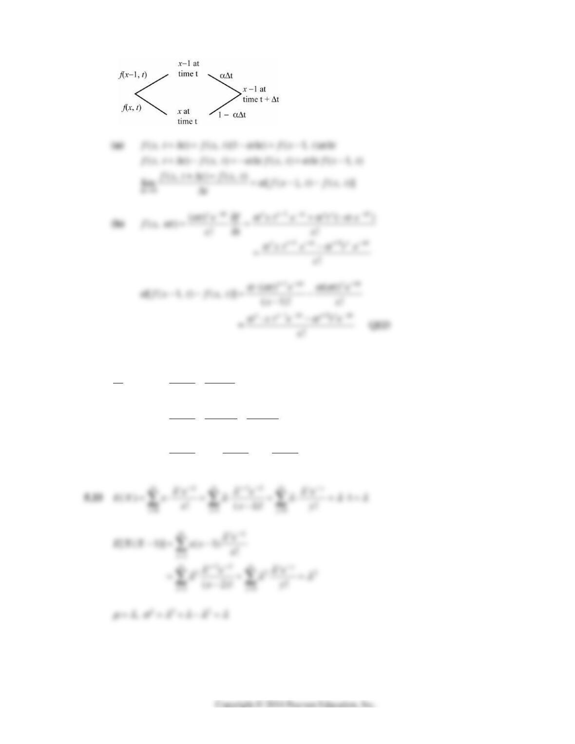
5.30
310
10 1000(0.000045) 0.045
(3; 10) 0.0075
666
e
p
Table II yields 0.0076
Chapter 5 69
5.31
5.32
xt
utdvedt
1
tx
v e du x t dt
1
1
2
0
0
11
!!(1)!
1
!(1)!(2)!
QED
!0! !
x
xt x t
xx
xt
x
xx
y
e
t e dt t e dt
xxx
ee tedt
xx x
eee
xy
λ
λλ
λλ
λ
λλλ
λ
λλ
λλλ
70 Mathematical Statistics, 8E
5.34 n,
0
θ
,
n
θ
λ
[1 ( 1)]
(1) (1)
11
tn
x
nn
tt
Me
ne e
nn
λ
λλ
1)
(
lim
t
e
n
e
λ
QED
5.36
11
0
1
1
0
1
1
1
0
11 1 1
()
() !!
() ()
!
() !
1
xx r
rxx
r
x
r
x
r
x
xx
r
r
x
r
rr r r
dex
rx x e e
dxx
x
rex
x
e
rxx
d
rr
d
λλ
λ
μλλ
λλλ
λ
λ
μλλ
λ
μλ
μ
μμ μλμ
λλ
1
01 2 0
1, 0, 1, 1 d
rd
μ
μ
μμλμ
λ
λ
31
2, 2 1r
μ
λμ λ
2
4
3, 3 1 3r
μ
λλ λλ
λ
μ
Chapter 5 71
5.39
1
1
!
() (1 )
!!( )!
(2)!
(1) (1 )
( 1)!( 1)!( )!
( 1)( )( )
jij
i
jij
i
xnxx
x
ij ij i j i j
ij i j
xnxx
x
ij i j i j
ij ij
ij
n
Exx xx xx n x x
n
nn xxnxx
nn
θθ θ θ
θθ θ θ θ θ
θθ
cov( , ) ( 1) ( )( )
ij ij i j
ij
xx nn n n
n
θθ θ θ
θθ
5.42 (a)
5
6(0.7) (0.3) 0.3025
5
(b) 0.3025
5.43 (a)
66
15 (0.4) (0.6) 5005(0.004096)(0.01008) 0.2066
6
(b) 0.2066
5.45 (a)
0.1529 0.0578 0.0098 0.2205
(b)
1 0.7794 0.2206
5.46 (a)
0.0285 0.0849 0.1734 0.2868
72 Mathematical Statistics, 8E
5.51
( 3) 1 (0;20,0.05) ( (1;20,0.05) (2;20,0.05)
1 0.3585 0.3774 0.1887 0.0754
Px b b b
Thus, there is only a 0.0754 chance of obtaining 3 or more failures if the manufacturer’s claim
is correct.
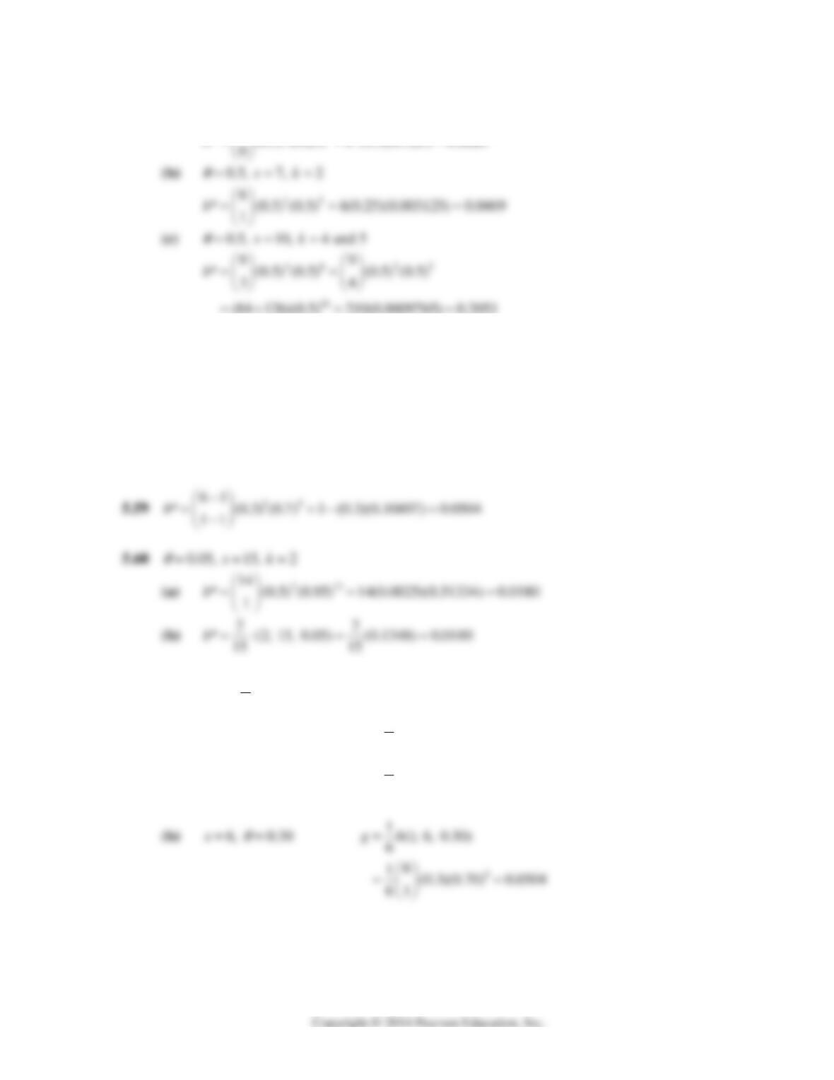
5.52 Using MINITAB software we first enter 13 and 18 in C1 and then give the commands:
MTB> CDF C1;
SUBC> BINOMIAL 100 .16667.
5.53 Using MINITAB with the number 12 entered into C1 and the commands:
MTB> CDF C1;
5.54 k = 6
(a)
450; 15
μ
σ
450 90
900
or 0.40 to 0.60
μ
μ
Chapter 5 73
5.57 (a)
0.5, 4, 1
xk
θ
13
3
* (0.5) (0.25) 1 (0.5)(0.125) 0.0625
b
5.58 (a)
0.75, 8, 5
xk
θ
53
7
* (0.75) (0.25) 35(0.2373)(0.015625) 0.1298
4
b
(b)
0.75, 15, 10
xk
θ
10 5
14
* (0.75) (0.25) 2002(0.05631)(0.0009765) 0.1101
9
b
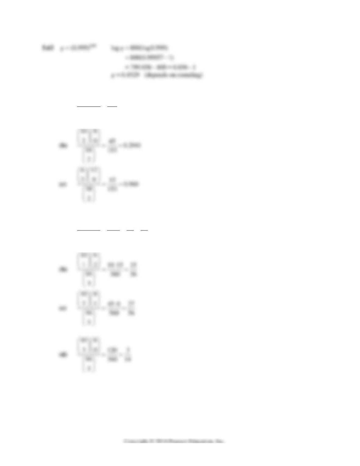
5.61
1
( ; 1, ) ( ; 1, )
gx bx
x
θθ
(a)
4, 0.75
x
θ
13
1(1; 4, 0.75)
4
4
1(0.75) (0.25) 0.0117
1
4
gb
74 Mathematical Statistics, 8E
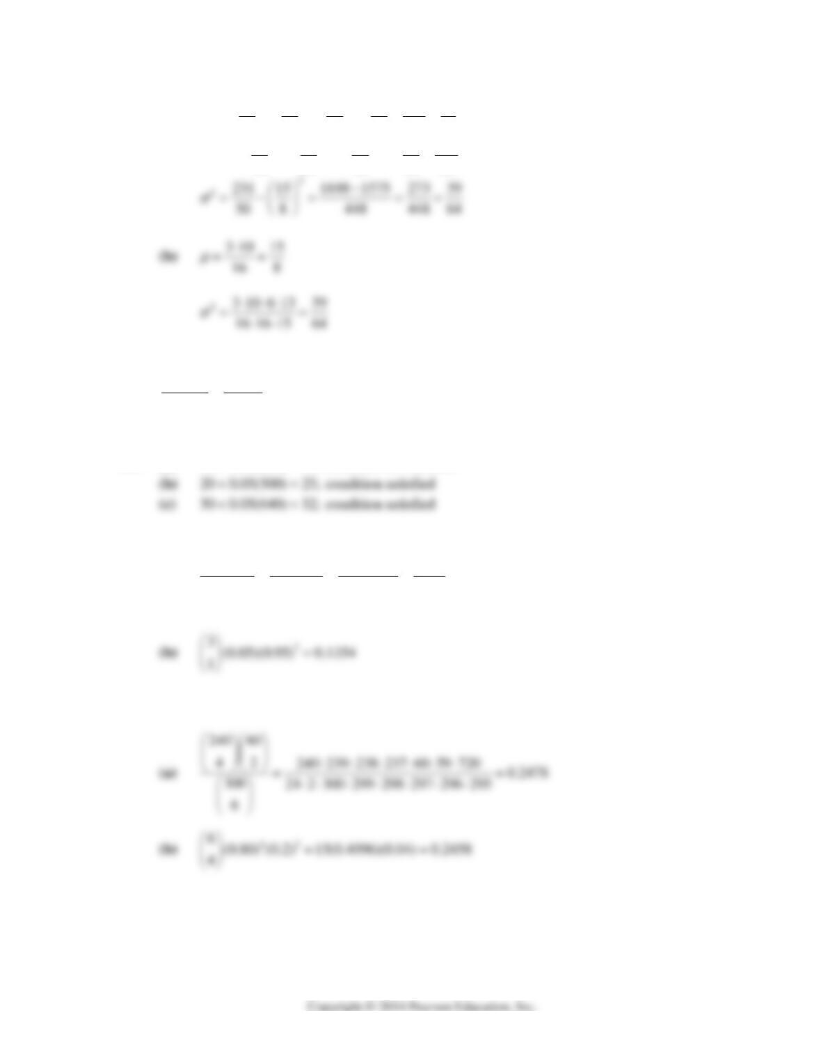
5.63 (a)
14 4
20 91 0.5948
18 153
2
5.64 (a)
10 6
03 120 2 1
16 560 56 28
3
Chapter 5 75
5.65 (a) 2 15 27 12 105 15
012 3
56 56 56 56 56 8
μ
22 2 2
2
2152712231
012 3
56 56 56 56 56
μ
5.66
96
23 36 20 0.2398
15 3003
5
5.67 (a) 12 0.05(200) 10; condition not satisfied
5.68 (a)
476
12 47675 6 285 0.1388
80 2 80 79 78 2054
3
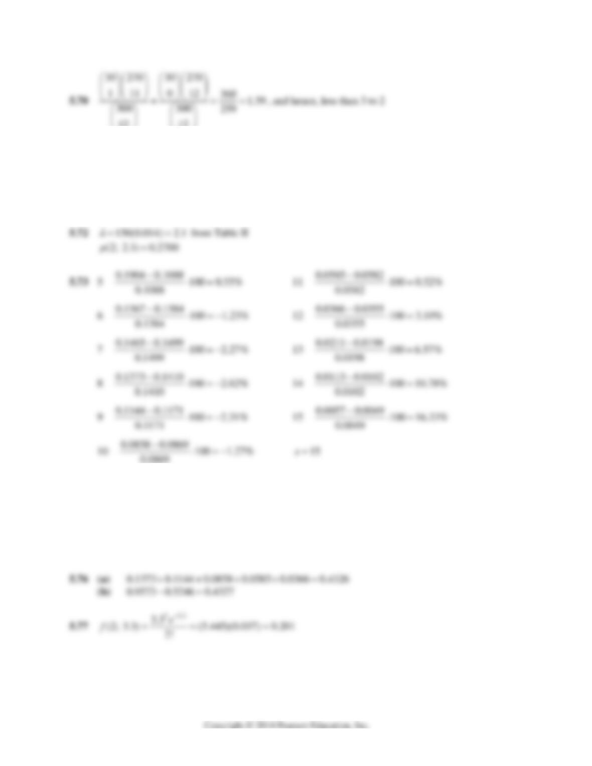
5.69 300, 240, 6, 4nM nx
76 Mathematical Statistics, 8E
12 12
5.71 Good 20n and 0.05
θ
excellent 100n and 10n
θ
(a) 125 20 and 0.10 0.05,also 12.5 10n
θ
; neither rule is satisfied
(b) 25 20, 0.04 0.05; good approximation
(c) 120 100, 6 10n
θ
; excellent approximation
(d) 0.06 0.05, 40 100; neither rule is satisfied
5.74 150(0.04) 6
λ
from Table II
(a) 0.1606
(b) 0.0025 0.0149 0.0446 0.892 0.1512
5.75 1000(0.0012) 1.2
λ
from Table II
(0) (1) (2) 0.3012 0.3614 0.2169 0.8795ppp
Chapter 5 77
5.78 (a)
01.8
(1.8)
(0; 1.8) 0.165
0!
e
f
(b)
1.8
1.8
(1; 1.8) 0.297
1
e
f
5.81 (a) (3; 5.2) 0.1293f
(b) 0.0220 0.0104 0.0045 0.0018 0.0007 0.0002 0.0001 0.0397
(c) 0.1681 0.1748 0.1515 0.4944
5.82 (a)
6994
0 100
(0; 100, 100, 6) 1000
100
h
(b) Using MINITAB software we enter 1 in C1 and give commands:
MTB> CDF C1;
SUBC? Binomial 100 .006.
obtaining K P(X LESS THAN OR = K)
1.5478
Thus, the approximate probability is 1 0.5478 0.4522
(c) Using the Poisson distribution having the mean 100 0.006 0.6, we obtain the
probability 1 0.5478 0.4522 from Table II.
5.83
36
10! (0.40) (0.50) (0.10) 840(0.064)(0.015625)(0.10) 0.0840
3! 6! 1!
78 Mathematical Statistics, 8E
5.86 (a)
15 7 3
410 1365 7 24 5 0.1798
25 25 24 23 22 21
5
(b)
15 7 3
311 455 7 3 120 0.1798
25 25 24 23 22 21
5
5.88 (rejection % defective 0.01) 0.10,P thus the producer’s risk is 0.10.
(rejection % defective 0.03) 0.95,P thus the consumer’s risk is 1 0.95 0.05.
5.91 (a) Producer’s risk = 1 value of L(p) when p = 0.10, or 0.17.
(b) LTPD = value of p for which L(p) = 0.05
5.92 If n = 10 and c = 1, we get the following from Table I.
5.93 If n = 15 and c = 2, we get the following from Table I.
5.94 If n = 8 and c = 0, we get the following from Table I.
Chapter 5 79
5.95 The AQL is the value of p for which ( ) 1 0.10 0.90Lp , or 0.07.
The LTPD is the value of p for which ( ) 0.10Lp or 0.33.
5.97 (a) If n = 10 and c = 0, we get the following from Table I.
p 0 0.05 0.10 0.15 0.20 0.25 0.30 0.35 0.40 0.45