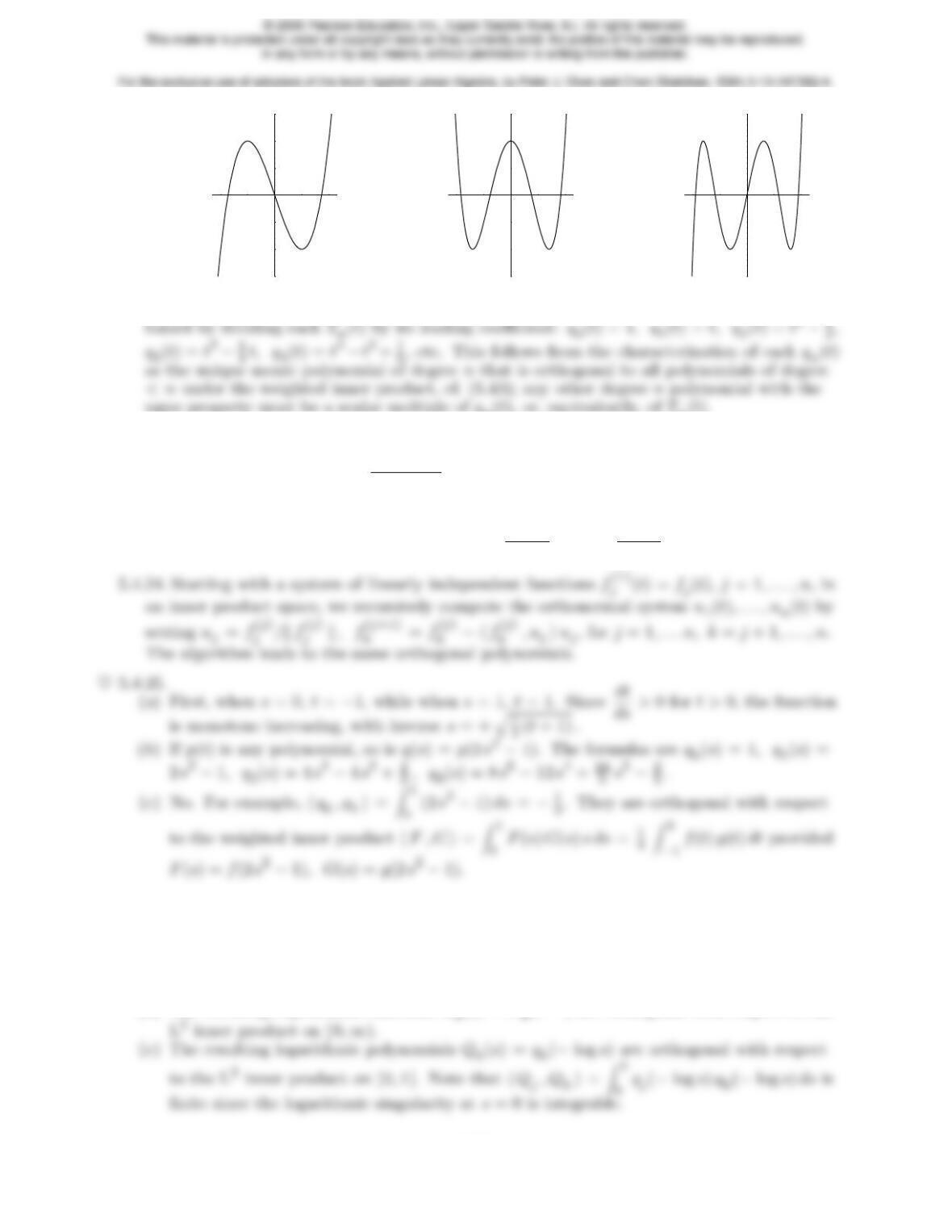
Mathematics Chapter 5 Is orthogonal to all polynomials of degree

-1 -0.5 0.5 1

-1.5

-1

-0.5

0.5

1

1.5

-1 -0.5 0.5 1

-1.5

-1

-0.5

0.5

1

1.5

-1 -0.5 0.5 1

-1.5

-1

-0.5

0.5

1

1.5

5.4.21. The Gram–Schmidt process will lead to the monic Chebyshev polynomials qn(t), ob-

5.4.22. A basis for the solution set is given by exand e2x. The Gram-Schmidt process yields

the orthogonal basis e2xand 2 (e3−1)

3 (e2−1) ex.

5.4.23. cos x, sin x, exform a basis for the solution space. Applying the Gram–Schmidt process,

we find the orthogonal basis cos x, sin x, ex+sinh π

πcos x−sinh π

πsin x.

5.4.26.

(a) By the change of variables formula for integrals, since ds =−e−tdt, then

hf , g i=Z∞

0f(t)g(t)e−tdt =Z1

0F(s)G(s)ds when f(t) = F(e−t), g(t) = G(e−t).

The change of variables does not map polynomials to polynomials.

(b) The resulting exponential functions Ek(t) = e

Pk(e−t) are orthogonal with respect to the

140

5.5.1. (a)v2,v4, (b)v3, (c)v2, (d)v2,v3, (e)v1, (f)v1,v3,v4.

5.5.2.

(a)0

B

@

−1

3

1

3

1

3

1

C

A, (b)0

B

@

4

7

−2

7

6

7

1

C

A≈0

B

@

.5714

−.2857

.8571 1

C

A, (c)0

B

@

7

9

11

9

1

9

1

C

A≈0

B

@

.7778

1.2222

.1111 1

C

A, (d)0

B

@

−1007

4225

301

4225

60

169

1

C

A≈0

B

@−.23833

.07123

.35503 1

C

A.

21

5.5.4. Orthogonal basis: 0

B

@−1

2

1

C

A,0

B

@

3

2

−5

2

1

C

A;

orthogonal projection: 2

30

B

@−1

2

1

C

A−4

50

B

@

3

2

−5

2

1

C

A=0

B

@

8

15

44

15

−4

3

1

C

A≈0

B

@

.5333

2.9333

−1.3333 1

C

A.

22

193

5.5.7. ( 1.3, .5, .2,−.1 )T.

♥5.5.8.

(a) The entries of c=ATvare ci=uT

iv=ui·v, and hence, by (1.11), w=Pv=Ac=

c1u1+···+ckuk, reproducing the projection formula (5.63).

141

(iv )0

B

@

1

9−2

92

90

−2

98

90−2

9

2

908

9−2

9

0−2

9−2

91

9

1

C

A

, (v)0

B

@

3

41

4

1

43

4−1

4

1

4−1

43

4−1

4

1

4−1

43

4

1

C

A

.

(c)PT= (AAT)T=AAT=P.

(d) The entries of ATAare the inner products ui·uj, and hence, by orthonormality, ATA=

I . Thus, P2= (AAT)(AAT) = AIAT=A AT=P. Geometrically, w=Pvis the

5.5.10. “1

2,−1

2,2”T.

5.5.11. (a)“−1

7,0”T, (b)“9

14 ,4

31 ”T, (c)“−4

7,1

30 ,2

7”T.

7,2,8

7,16

7”T.

5.5.15.

(a)p1(t) = 14 + 7

2t, p2(t) = p3(t) = 14 + 7

2t+1

14 (t2−2);

(b)p1(t) = .285714 + 1.01429t, p2(t) = .285714 + 1.01429 t−.0190476 (t2−4),

hq1,q2i=1

n

X

i= 1

ti(t2

i−t2) = t3−t t2= 0,

hq1,q3i=1

n

X

i= 1

ti0

@t3

i−t4

t2ti1

A=t4−t4

t2t2= 0,

5.5.17.

(a)p4(t) = 14 + 7

2t+1

14 (t2−2) −5

12 “t4−31

7+72

35 ”;

(b)p4(t) = .2857 + 1.0143 t−.019048 (t2−4) −.008333 (t3−7t) + .011742 “t4−67

7t2+72

7”;

(c)p4(t) = 100 + 80

7−20

21 (t2−4) −5

66 “t4−67

7t2+72

7”.

5.5.18. Because, according to (5.65), the kth Gram-Schmidt vector belongs to the subspace

spanned by the first kof the original basis vectors.

♥5.5.19.

(a) Since ti=t0+i h, we have t=t0+1

2nh and so si=“i−1

2n”h. In particular,

5.5.21. For simplicity, we assume ker A={0}. According to Exercise 5.3.33, orthogonalizing

the basis vectors for rng Ais the same as factorizing A=QR where the columns of Qare

the orthonormal basis vectors, while Ris a nonsingular upper triangular matrix. The for-

143

5.5.23. The solutions are, of course, the same:

(a)Q=0

B

@

.30151 .79455

.90453 −.06356

−.30151 .60386 1

C

A, R = 3.31662 −.90453

0 2.86039 !,x= .06667

.91111 !;

(b)Q=0

B

@

.8−.43644

.4.65465

.2−.43644

.4.43644

1

C

A, R = 5 0

0 4.58258 !,x= −.04000

−.38095 !;

♦5.5.24. The second method is more efficient! Suppose the system is Ax=bwhere Ais an

m×nmatrix. Constructing the normal equations requires mn2multiplications and

(m−1)n2≈mn2additions to compute ATAand an additional nm multiplications and

n(m−1) additions to compute ATb. To solve the normal equations ATAx=ATbby Gaus-

♦5.5.25.

(a) If A=Qhas orthonormal columns, then

kQx⋆−bk2=kbk2− kQTbk2=

m

X

i= 1

b2

i−

n

X

i= 1

(ui·b)2.

144

5.5.27.

(a)P=0

B

@

.25 −.25 −.35 .05

−.25 .25 .35 −.05

−.35 .35 .49 −.07

.05 −.05 −.07 .01

1

C

A,Pv=0

B

@

.25

−.25

−.35

.05

1

C

A;

(b)P=0

B

@

1

3−1

301

3

−1

37

9−2

91

9

0−2

91

9−2

9

1

31

9−2

97

9

1

C

A

,Pv=0

B

@

1

3

−1

3

0

1

3

1

C

A

;

5.5.28. Both are the same quadratic polynomial: 1

5+4

7“−1

2+3

2t2”=−3

35 +6

7t2.

5.5.29.

Quadratic: 1

5+2

5(2t−1)+ 2

7(6t2−6t+1) = 3

35 −32

35 t+12

7t2=.08571−.91429t+1.71429t2;

Cubic: 1

5+2

5(2t−1)+ 2

7(6t2−6t+1) + 1

10 (20t3−30t2+12t−1) = −1

70 +2

7t−9

7t2+2t3=

−.01429 + .2857t−1.2857t2+ 2t3.

145

(b)

0.5 1 1.5 2 2.5 3

0.2

0.4

0.6

0.8

1

The maximum error is .0504655 at the ends t= 0, π.

♠5.5.33. .459698 + .427919 (2t−1) −.0392436 (6t2−6t+ 1) −.00721219 (20t3−30t2+ 12t−1) =

−.000252739 + 1.00475 t−.0190961 t2−.144244 t3.

♠5.5.34.

5.5.35.

(a)3

2−10

3“t−3

4”+35

4“t2−4

3t+2

5”=15

2−15t+35

4t2; it gives the smallest value to

5t3.

(c)

0.2 0.4 0.6 0.8 1

5

10

15

20

25

30

(d) Both do a reasonable job approximating from t=.2 to 1, but can’t keep close near the

singularity at 0, owing to the small value of the weight function w(t) = t2there. The

cubic does a marginally better job near the singularity.

246 8

5.6.1. (a)W⊥has basis 0

B

@

1

3

1

0

1

C

A,0

B

@−1

3

0

1

C

A, dim W⊥= 2; (b)W⊥has basis 0

B

@

−1

2

−5

4

1

C

A,

146

dim W⊥= 1; (c)W⊥has basis 0

B

@−2

1

01

C

A,0

B

@−3

0

11

C

A, dim W⊥= 2; (d)W⊥has basis 0

B

@

2

1

11

C

A,

dim W⊥= 1; (e)W⊥={0}, dim W⊥= 0.

5.6.4. (a)w=0

@

3

10

−1

10 1

A,z=0

@

7

10

21

10 1

A; (b)w=0

B

@

−1

5

8

25

−31

25

1

C

A,z=0

B

@

−6

5

42

25

−6

25

1

C

A; (c)w=0

B

@

1

3

−1

3

−1

3

1

C

A,

z=0

B

@

2

3

1

3

1

3

1

C

A; (d)w=0

B

@

2

7

−3

7

−1

7

1

C

A,z=0

B

@

5

7

3

7

1

7

1

C

A; (e)w=0

B

@

4

11

−1

11

1

11

1

C

A

,z=0

B

@

7

11

1

11

−1

11

13

1

C

A

.

5.6.6. For the weighted inner product, the orthogonal complement W⊥is the set of all vectors

v= ( x, y, z, w )Tthat satisfy the linear system

hv,w1i=x+ 2y+ 4w= 0,hv,w2i=x+ 2y+ 3 z−8w= 0.

5.6.7. (a)hp , q i=Z1

−1p(x)q(x)dx = 0 for all q(x) = a+bx +cx2, or, equivalently,

Z1

−1p(x)dx =Z1

−1x p(x)dx =Z1

−1x2p(x)dx = 0. Writing p(x) = a+b x +c x2+d x3+e x4,

147

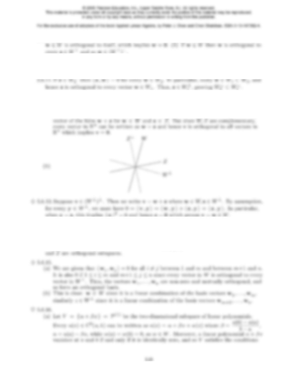
5.6.9. (a) If w∈W∩W⊥then w∈W⊥must be orthogonal to every vector in Wand so

5.6.10. (a) The only element orthogonal to all v∈Vis 0, and hence V⊥contains only the zero

vector. (b) Every v∈Vis orthogonal to 0, and so belongs to {0}⊥.

5.6.12.

(a) We are given that dim W+ dim Z=nand W∩Z={0}. Now, dim W⊥=n−dim W,

dim Z⊥=n−dim Zand hence dim W⊥+ dim Z⊥=n. Furthermore, if v∈W⊥∩Z⊥

then vis orthogonal to all vectors in both Wand Z, and hence also orthogonal to any

5.6.14. Every w∈Wcan be written as w=

k

X

i= 1

aiwi; every z∈Zcan be written as

z=

l

X

j= 1

bjzj. Then, using bilinearity, hw,zi=

k

X

i= 1

l

X

j= 1

aibjhwi,zji= 0, and hence W

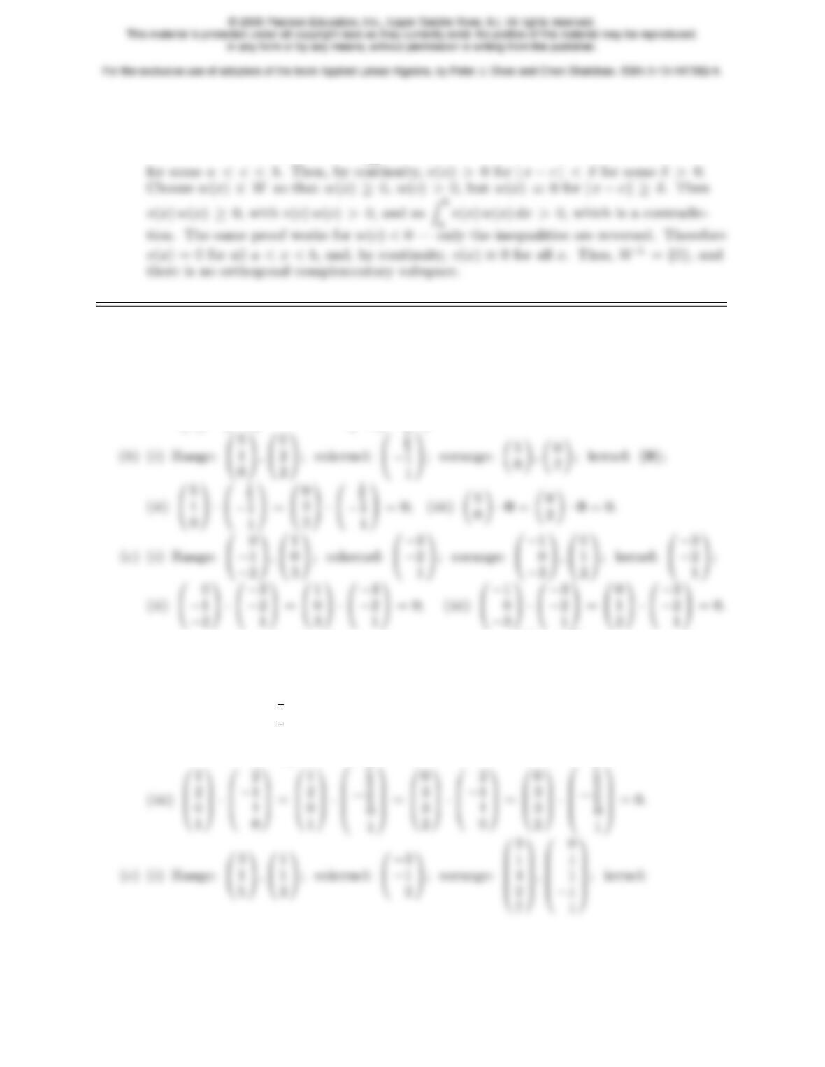
for it to be a complementary subspace to W.

(b) The only continuous function which is orthogonal to all functions in Wis the zero func-

tion. Indeed, suppose hv , w i=Zb

5.6.17. Note: To show orthogonality of two subspaces, it suffices to check orthogonality of their

respective basis vectors.

(a) (i) Range: 1

2!; cokernel: −2

1!; corange: 1

−2!; kernel: 2

1!;

(ii ) 1

2!· −2

1!= 0; (iii ) 1

−2!· 2

1!= 0.

(d) (i) Range: 0

B

@

1

−1

01

C

A,0

B

@

2

1

31

C

A; cokernel: 0

B

@−1

−1

11

C

A; corange: 0

B

@

1

2

0

1

C

A,0

B

@

0

3

2

1

C

A;

kernel: 0

B

@

2

−1

1

0

1

C

A,0

B

@

1

3

−2

3

0

1

C

A; (ii )0

B

@

1

−1

01

C

A·0

B

@−1

−1

11

C

A=0

B

@

2

1

31

C

A·0

B

@−1

−1

11

C

A= 0;

149

0

B

@

−1

1

0

1

C

A

,0

B

@

−1

1

0

1

C

A

,0

B

@

−2

−1

0

1

C

A

; (ii )0

B

@

3

1

51

C

A·0

B

@−3

−1

21

C

A=0

B

@

1

21

C

A·0

B

@−3

−1

21

C

A= 0; (iii )0

B

@

3

1

4

2

1

C

A·0

B

@

−1

1

0

1

C

A

(f) (i) Range: 0

B

@

1

−2

−3

1

C

A,0

B

@

3

1

5

−4

1

C

A; cokernel: 0

B

@

−1

−2

1

0

1

C

A,0

B

@

1

0

1

C

A; corange: 0

B

@

1

3

0

−2

1

C

A,0

B

@

0

7

2

−1

1

C

A;

kernel: 0

B

@

6

7

−2

7

1

C

A,0

B

@

11

7

1

7

0

1

C

A;

0

B

@

−1

2

−1

1

C

A,0

B

@

0

1

0

1

C

A; kernel: 0

B

@

2

1

0

1

C

A,0

B

@

−1

0

1

C

A; (ii )0

B

@

−1

2

−3

1

−2

1

C

A·0

B

@

−11

−4

1

0

1

C

A

=0

B

@

−1

2

−3

1

−2

1

C

A·0

B

@

−1

0

1

0

1

C

A

=

0

B

@

−1

2

−3

1

−2

1

C

A·0

B

@

−20

−9

0

1

C

A

=0

B

@

2

−5

2

−3

−5

1

C

A·0

B

@

−11

−4

1

0

1

C

A

=0

B

@

2

−5

2

−3

−5

1

C

A·0

B

@

−1

0

1

0

1

C

A

=0

B

@

2

−5

2

−3

−5

1

C

A·0

B

@

−20

−9

0

1

C

A

= 0;

5.6.18.

(a) The compatibility condition is 2

3b1+b2= 0 and so the cokernel basis is “2

3,1”T.

150

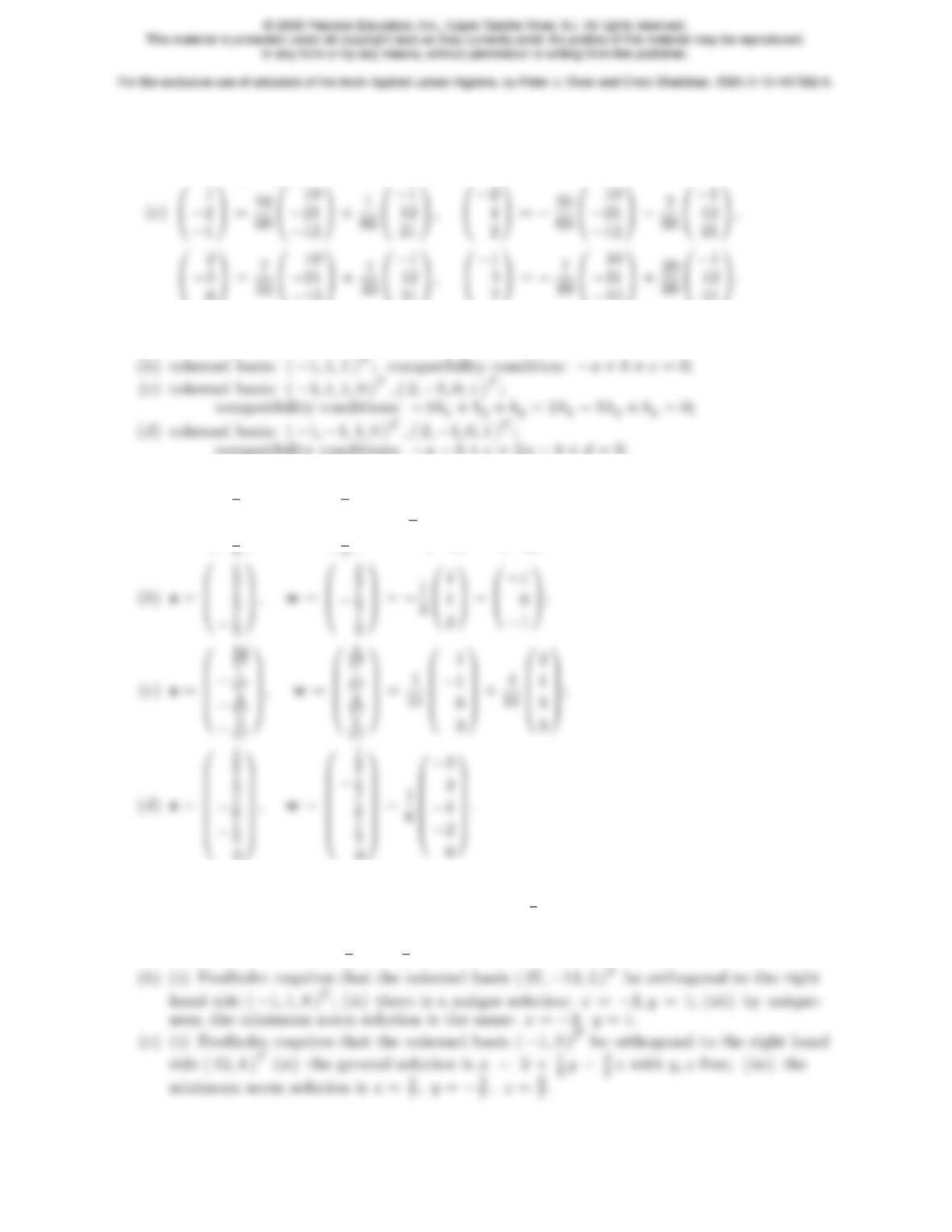
5.6.19. (a)0

B

@

1

−2

2

−1

1

C

A,0

B

@

0

1

3

1

C

A; (b)0

B

@

10

−21

−12 1

C

A,0

B

@−1

12

21 1

C

A;

5.6.20.

(a) Cokernel basis: ( 1,−1,1 )T; compatibility condition: 2 a−b+c= 0;

5.6.21.

(a)z=0

B

@

1

2

0

−1

1

C

A,w=0

B

@

1

2

0

1

C

A=−3

20

B

@

1

−2

1

C

A+0

B

@

2

−3

2

1

C

A;

0

5.6.22.

(a) (i) Fredholm requires that the cokernel basis “1

2,1”Tbe orthogonal to the right hand

side ( −6,3 )T; (ii ) the general solution is x=−3 + 2ywith yfree; (iii ) the minimum

norm solution is x=−3

5, y =6

5.

151

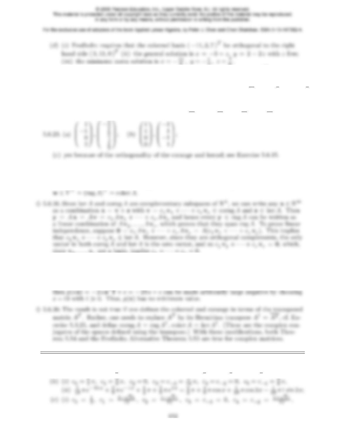
6, y =−1

3, z =7

6.

(e) (i) Fredholm requires that the cokernel basis ( −10,−9,7,0 )T,( 6,4,0,7 )Tbe orthogo-

nal to the right hand side ( −8,5,−5,4 )T; (ii ) the general solution is x1= 1 −t, x2=

3+2t, x3=twith tfree; (iii ) the minimum norm solution is x1=11

6, x2=4

3, x3=−5

6.

(f) (i) Fredholm requires that the cokernel basis ( −13,5,1 )Tbe orthogonal to the right

hand side ( 5,13,0 )T; (ii ) the general solution is x= 1 + y+w, z = 2 −2wwith y, w

free; (iii ) the minimum norm solution is x=9

11 , y =−9

11 , z =8

11 , w =7

11 .

5.6.24. If Ais symmetric, ker A= ker AT= coker A, and so this is an immediate consequence of

Theorem 5.55.

♦5.6.25. Since rng A= span {v1, . . . , vn}=V, the vector wis orthogonal to Vif and only if

5.6.27. False. The resulting basis is almost never orthogonal.

5.6.28. False. See Example 5.60 for a counterexample.

♦5.6.29. If f6∈ rng K, then there exists x∈ker K= coker Ksuch that xTf=x·f=b6= 0. But

5.7.1.

(a) (i)c0= 0, c1=−1

2i, c2=c−2= 0, c3=c−1=1

2i,(ii )1

2ie−ix−1

2ieix= sin x;

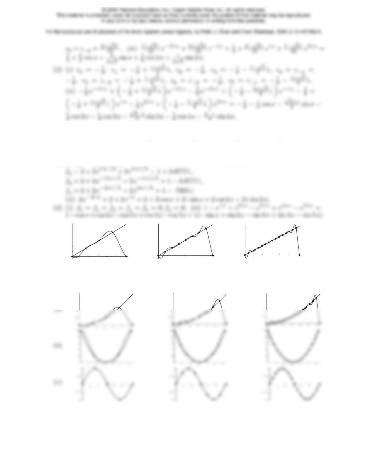
5.7.2.

(a) (i)f0=f3= 2, f1=−1, f2=−1.(ii )e−ix+eix= 2 cos x;

(b) (i)f0=f5= 1, f1= 1 −√5, f2= 1 + √5, f3= 1 + √5, f4= 1 −√5 ;

(ii )e−2 i x−e−ix+ 1 −eix+e2 i x= 1 −2 cos x+ 2 cos 2x;

(c) (i)f0=f5= 6, f1= 2 + 2e2πi/5+ 2e−4πi/5= 1 + .7265 i ,

♠5.7.3.

12 3 4 5 6

1

2

3

4

5

6

12 3 4 5 6

1

2

3

4

5

6

12 3 4 5 6

1

2

3

4

5

6

The interpolants are accurate along most of the interval, but there is a noticeable problem

near the endpoints x= 0,2π. (In Fourier theory, [16,47], this is known as the Gibbs phe-

nomenon.)

♠5.7.4.

30

40

30

40

20

30

40

153

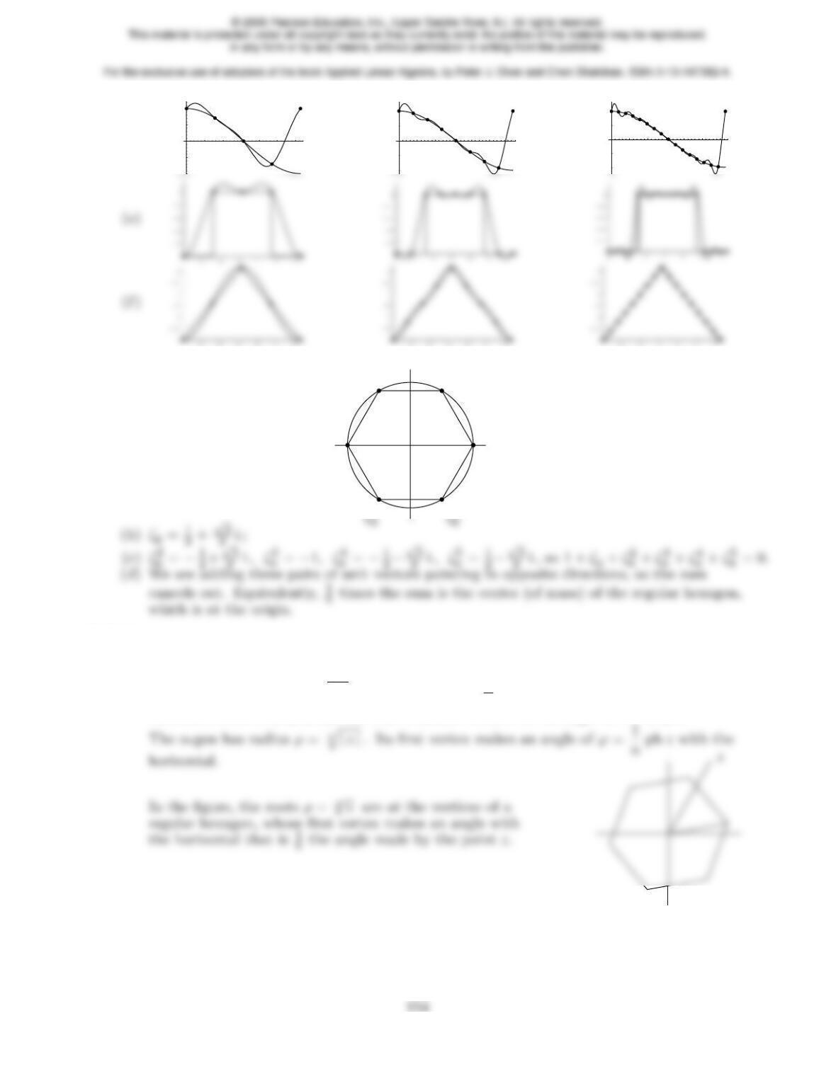
(d)

12 3 4 5 6

-0.5

0.5

1

12 3 4 5 6

-1

-0.5

0.5

1

12 3 4 5 6

-1

-0.5

0.5

1

5.7.5.

(a)ζ0

6= 1

ζ6

ζ2

6

ζ3

6=−1

♦5.7.6.

(a) The roots all have modulus |ζk|= 1 and phase ph ζk= 2 πk/n. The angle between

successive roots is 2π/n. The sides meet at an angle of π−2π/n.

(b) Every root has modulus n

q|z|and the phases are 1

n“ph z+ 2πk ”, so the angle between

successive roots is 2π/n, and the sides continue to meet at an angle of π−2π/n.

♦5.7.7.

(a) (i) i ,−i ; (ii )e2πk i/5for k= 1,2,3 or 4; (iii )e2πk i/9for k= 1,2,4,5,7 or 8;

(b)e2πk i/n whenever kand nhave no common factors, i.e., kis relatively prime to n.

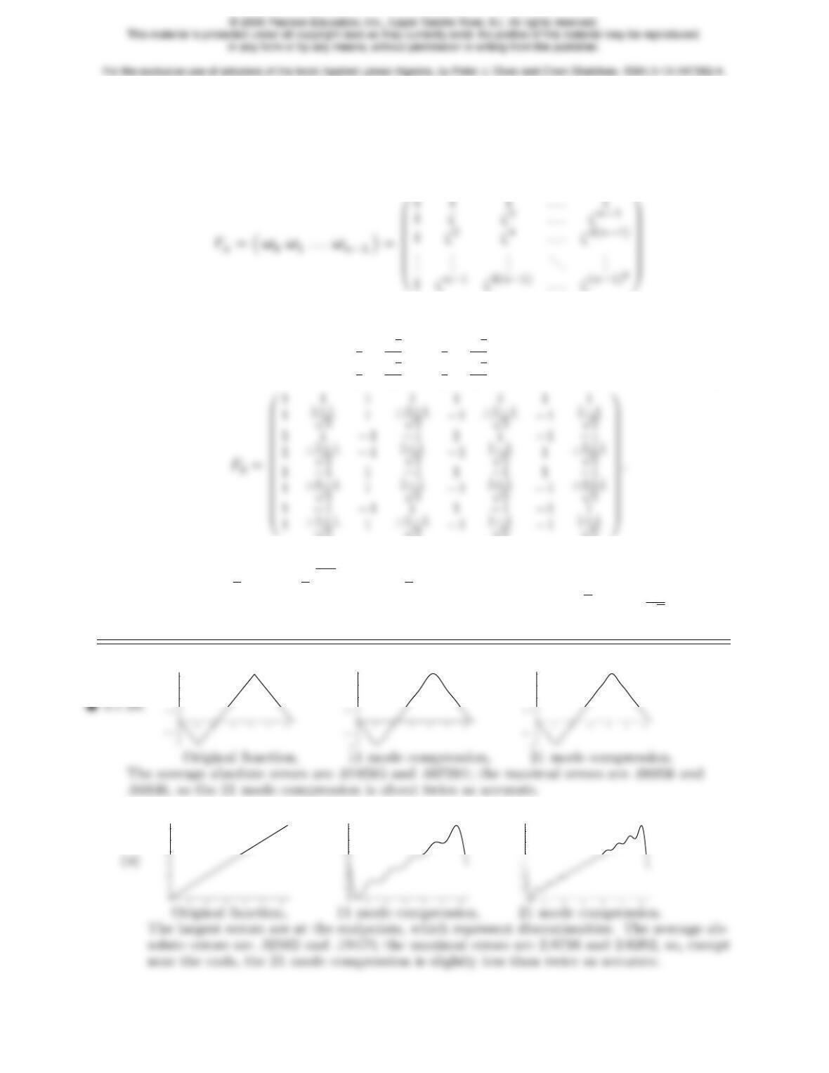
5.7.8. (a) Yes, the discrete Fourier coefficients are real for all n. (b) A function f(x) has real

discrete Fourier coefficients if and only if f(xk) = f(2π−xk) on the sample points x0, . . . , xn−1.

In particular, this holds when f(x) = f(2π−x).

♥5.7.9. (a) In view of (2.13), formula (5.91) is equivalent to matrix multiplication f=Fnc,

where

0

1

is the n×nmatrix whose columns are the sampled exponential vectors (5.90). In particular,

F2= 1 1

1−1!, F3=0

B

@

1 1 1

1−1

2+√3

2i−1

2−√3

2i

1−1

2−√3

2i−1

2+√3

2i

1

C

A, F4=0

B

@

1 1 1 1

1 i −1−i

1−1 1 −1

1−i−1 i

1

C

A,

(b) Clearly, if f=Fnc, then c=F−1

nf. Moreover, formula (5.91) implies that the (i, j)

entry of F−1

nis 1

nζ−i j

n=1

nζi j

n, which is 1

ntimes the complex conjugate of the (j, i) entry

of Fn. (c) By part (b), U−1

n=√n F −1

n=1

√nF†

n=U†

n.

1

1.5

2

1

1.5

2

1

1.5

2

♠5.7.11.

5

6

5

6

5

6

155

(b)

12 3 4 5 6

20

40

60

80

12 3 4 5 6

20

40

60

80

12 3 4 5 6

20

40

60

80

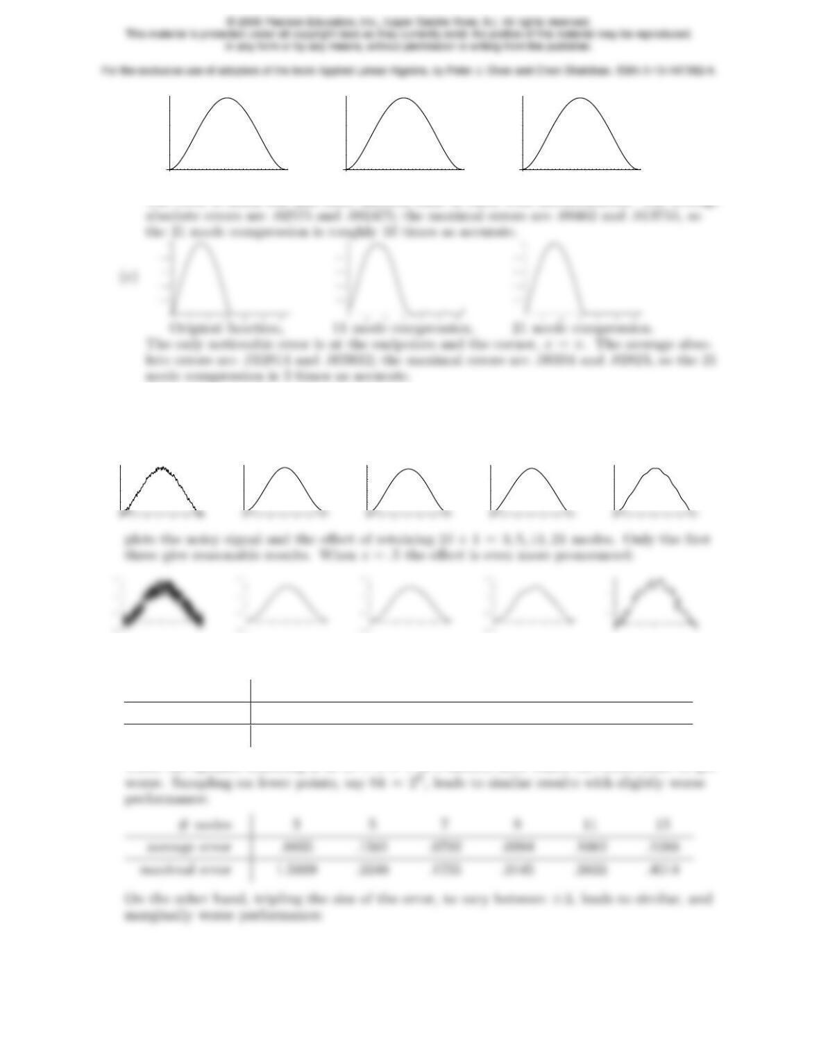
Original function, 11 mode compression, 21 mode compression.

The error is much less and more uniform than in cases with discontinuities. The average

♣5.7.12. l= 4, 27, 57.

♣5.7.13. Very few are needed. In fact, if you take too many modes, you do worse! For example,

if ε=.1,

0.5

1

1.5

2

0.5

1

1.5

2

0.5

1

1.5

2

0.5

1

1.5

2

0.5

1

1.5

2

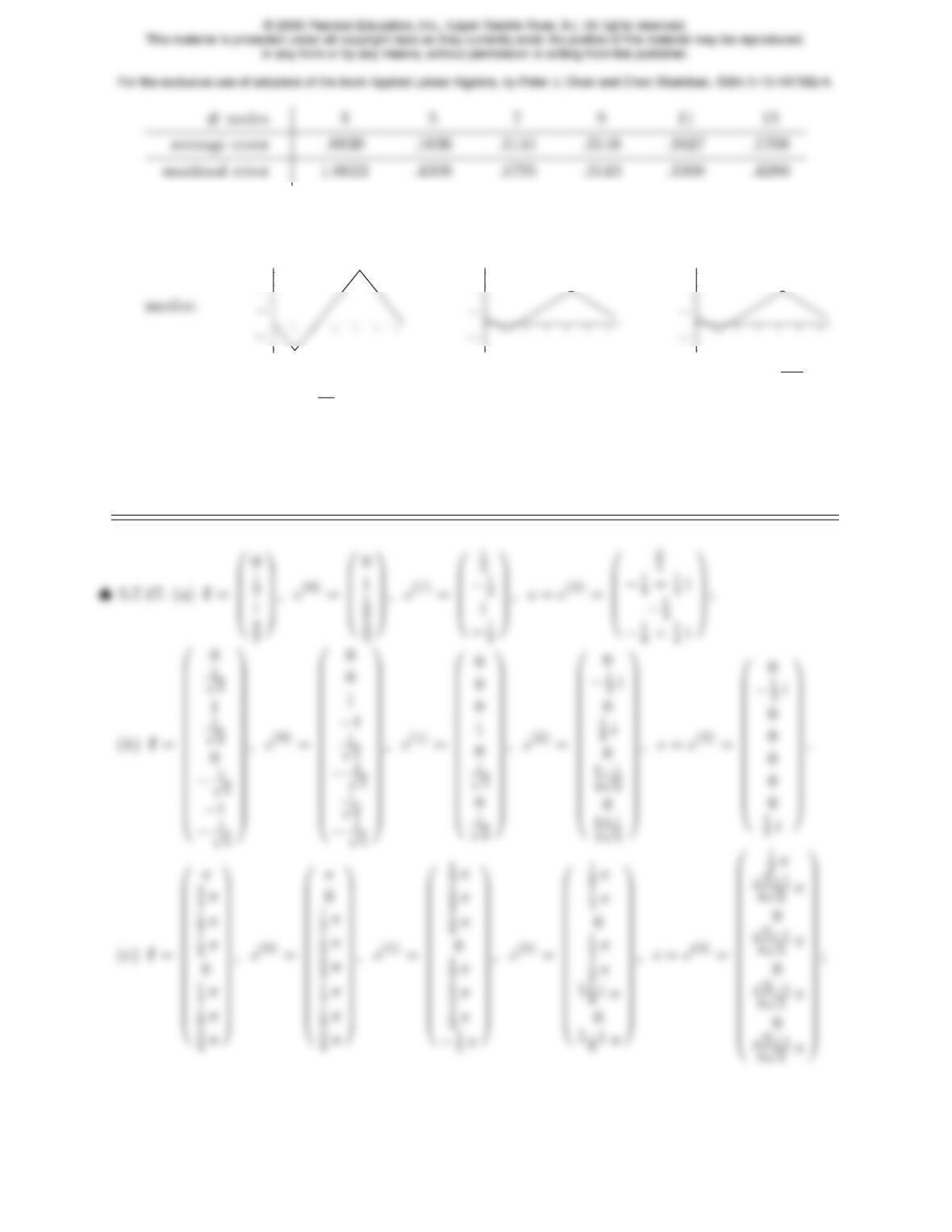
♠5.7.14. For noise varying between ±1, and 256 = 28sample points, the errors are

# nodes 3 5 7 9 11 13

average error .8838 .1491 .0414 .0492 .0595 .0625

maximal error 1.5994 .2687 .1575 .1357 .1771 .1752

Thus, the optimal denoising is at 2l+ 1 = 7 or 9 modes, after which the errors start to get

156

Note: the numbers will slightly vary each time the random number generator is run.

♣5.7.15. The “compressed” function differs significantly from original signal. The following plots

are the function, that obtained by retaining the first l= 11 modes, and then the first l= 21

-1

1.5

2

-1

1.5

2

-1

1.5

2

5.7.16. True for the odd case (5.103), but false for the even case (5.104). Since ω−k=ωk,

when fis real, c−k=ck, and so the terms c−ke−ik x +ckeik x = 2 Re ckeik x combine

to form a real function. Moreover, the constant term c0, which equals the average sample

value of f, is also real. Thus, all terms in the odd sum pair up into real functions. How-

ever, in the even version, the initial term c−me−im x has no match, and remains, in gen-

eral, complex. See Exercise 5.7.1 for examples.

157

(d)f= ( 1,1,1,1,1,1,0,0,0,0,0,0,0,0,0,0 )T,

c(0) = ( 1,0,1,0,1,0,0,0,1,0,1,0,1,0,0,0 )T,

♠5.7.18.

(a)c=0

B

@

1

−1

1

−1

1

C

A,f(0) =0

B

@

1

−1

1

C

A,f(1) =0

B

@

2

0

−2

0

1

C

A,f=f(2) =0

B

@

0

4

0

1

C

A;

−1

0

3

0

3

√2(1 −i )

1

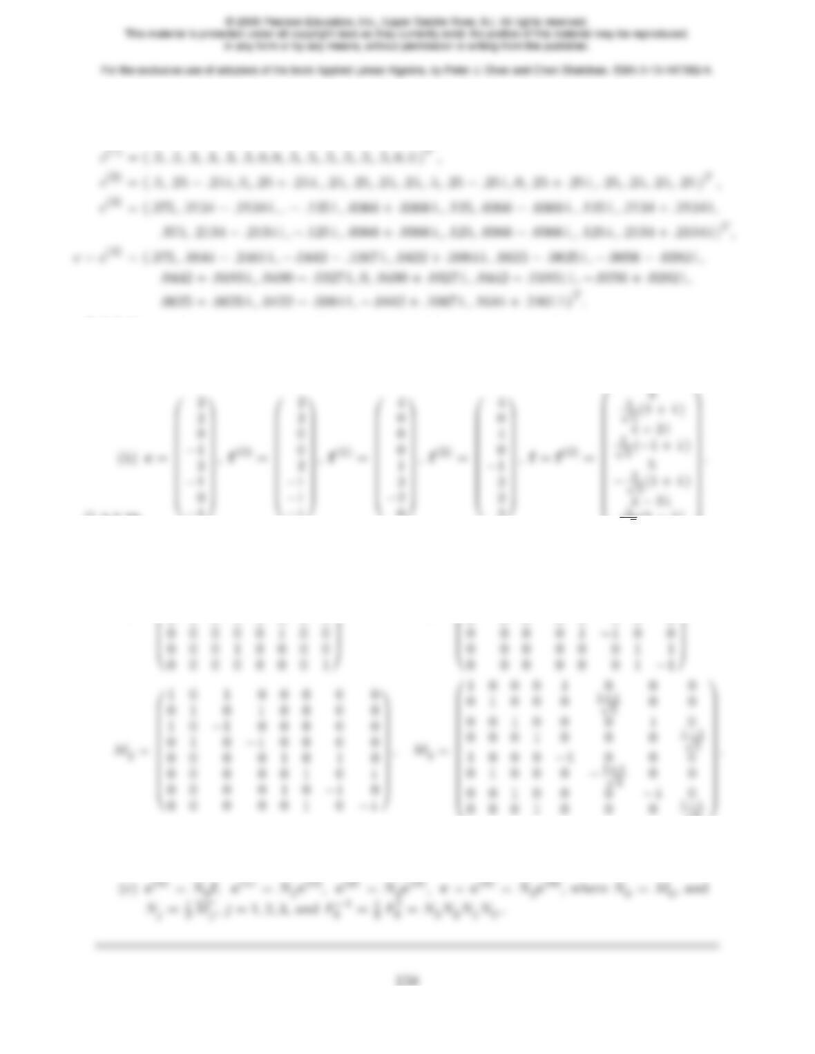
♥5.7.19.

(a)

M0=

0

B

10000000

00001000

00100000

00000010

01000000

1

C

, M1=

0

B

1 1 0 0 0 0 0 0

1−1 0 0 0 0 0 0

0 0 1 1 0 0 0 0

0 0 1 −1 0 0 0 0

0 0 0 0 1 1 0 0

1

C

,

(b) Because, by composition, f=M3M2M1M0c. On the other hand, according to Exercise

5.7.9, f=F8c, and so M3M2M1M0c=F8c. Since this holds for all c, the coefficient

matrices must be equal: F8=M3M2M1M0.