Solutions — Chapter 4
4.1.1. We need to minimize (3x−1)2+ (2 x+ 1)2= 13 x2−2x+ 2. The minimum value of 25
13
occurs when x=1
13 .
4.1.2. Note that f(x, y)≥0; the minimum value f(x?, y?) = 0 is achieved when
x?=−5
7, y?=−4
7.
4.1.3. (a) ( −1,0 )T, (b) ( 0,2 )T, (c)“1
2,1
2”T, (d)“−3
2,3
2”T, (e) ( −1,2 )T.
4.1.4. Note: To minimize the distance between the point ( a, b )Tto the line y=mx +c:
4.1.5.
(a) Uniqueness is assured in the Euclidean norm. (See the following exercise.)
(b) Not unique. For instance, in the ∞norm, every point on the x-axis of the form (x, 0)
♥4.1.6.
(a) The closest point vis found by dropping a
perpendicular from the point to the line:
b
v
θ
4.1.7. This holds because the two triangles in the figure are congruent. According to Exercise
4.1.6(c), when kak=kbk= 1, the distance is |sin θ|where θis the angle between a,b, as
a
b
θ
4.1.8.
4.1.10.
(a) Let v?be the minimizer. Since x2is a montone, strictly increasing function for x≥0,
4.1.11.
(a) Assume V6={0}, as otherwise the minimum and maximum distance is kbk. Given any
06=v∈V, by the triangle inequality, kb−tvk ≥ |t| kvk − kbk → ∞ as t→ ∞, and
hence there is no maximum distance.
4.2.1. x=1
2, y =1
2, z =−2 with f(x, y, z) = −3
2. This is the glboal minimum because the
coefficient matrix 0
B
@
110
131
0111
C
Ais positive definite.
105
4.2.5.
(a)p(x) = 4x2−24xy + 45y2+x−4y+ 3; minimizer: x?=“1
24 ,1
18 ”T≈(.0417, .0556 )T;
minimum value: p(x?) = 419
144 ≈2.9097.
(b)p(x) = 3x2+ 4xy +y2−8x−2y; no minimizer since Kis not positive definite.
(c)p(x) = 3x2−2xy + 2xz + 2y2−2y z + 3z2−2x+ 4 z−3; minimizer: x?=
“7
12 ,−1
6,−11
12 ”T≈(.5833,−.1667,−.9167 )T; minimum value: p(x?)=−65
12 =−5.4167.
4.2.6. n= 2: minimizer x?=“−1
6,−1
6”T; minimum value −1
6.
n= 3: minimizer x?=“−5
28 ,−3
14 ,−5
28 ”T; minimum value −2
7.
n= 4: minimizer x?=“−2
11 ,−5
22 ,−5
22 ,−2
11 ”T; minimum value −9
22 .
♦4.2.9. Let x?=K−1fbe the minimizer. When c= 0, according to the third expression in
(4.12), p(x?)=−(x?)TKx?≤0 because Kis positive definite. The minimum value is 0 if
and only if x?=0, which occurs if and only if f=0.
4.2.10. First, using Exercise 3.4.20, we rewrite q(x)=xTKxwhere K=KTis symmetric. If
Kis positive definite or positive semi-definite, then the minimum value is 0, attained when
x?=0(and other points in the semi-definite cases). Otherwise, there is at least one vector
vfor which q(v)=vTKv=a < 0. Then q(tv)=t2acan be made arbitrarily large
negative for tÀ0; in this case, there is no minimum value.
4.3.1. Closest point: “6
7,38
35 ,36
35 ”T≈(.85714,1.08571,1.02857 )T; distance: 1
√35 ≈.16903.
4.3.2.
4.3.3. “7
9,8
9,11
9”T≈(.7778, .8889,1.2222 )T.
4.3.4.
4.3.5. Since the vectors are linearly dependent, one must first reduce to a basis consisting of the
first two. The closest point is “1
2,1
2,1
2,1
2”Tand the distance is 3.
4.3.6.
(i) 4.3.4: (a) Closest point: “3
2,3
2,3
2,3
2”T; distance: q7
4.
4.3.5: Closest point: “3
11 ,13
22 ,−4
11 ,−1
22 ”T≈(.2727, .5909,−.3636,−.0455 )T;
distance: q155
22 ≈2.6543.
4.3.5: Closest point: “26
259 ,−107
259 ,−292
259 ,159
259 ”T≈(.1004,−.4131,1.1274, .6139 )T;
distance: 8q143
259 ≈5.9444.
4.3.7. v=“6
5,3
5,3
2,3
2”T= ( 1.2, .6,1.5,1.5 )T.
4.3.8. (a)q8
3; (b)7
√6.
107
♦4.3.10.
(a) The quadratic function to be minimized is
p(x) =
n
X
i= 1 kx−aik2=nkxk2−2x·0
@
n
X
i= 1
ai1
A+
n
X
i= 1 kaik2,
4.3.11. In general, for the norm based on the positive definite matrix C, the quadratic function
to be minimized is
p(x) =
n
X
i= 1 kx−aik2=nkxk2−2nhx,bi+n c =n“xTCx−2xTCb+c”,
4.3.12. The Cauchy–Schwarz inequality guarantees this.
♦4.3.13.
4.3.14. (a)x=1
15 , y =41
45 ; (b)x=−1
25 , y =−8
21 ; (c)u=2
3, v =5
3, w = 1;
65 1
0
941 1
−.0990 1
4.3.16. The solution is ( 1,0,3 )T. If Ais nonsingular, then the least squares solution to the sys-
tem Ax=bis given by x?=K−1f= (ATA)−1ATb=A−1A−TATb=A−1b, which
4.3.17. The solution is x?= ( −1,2,3 )T. The least squares error is 0 because b∈rng Aand so
x?is an exact solution.
♦4.3.18.
(a) This follows from Exercise 3.4.31 since f∈corng A= rng K.
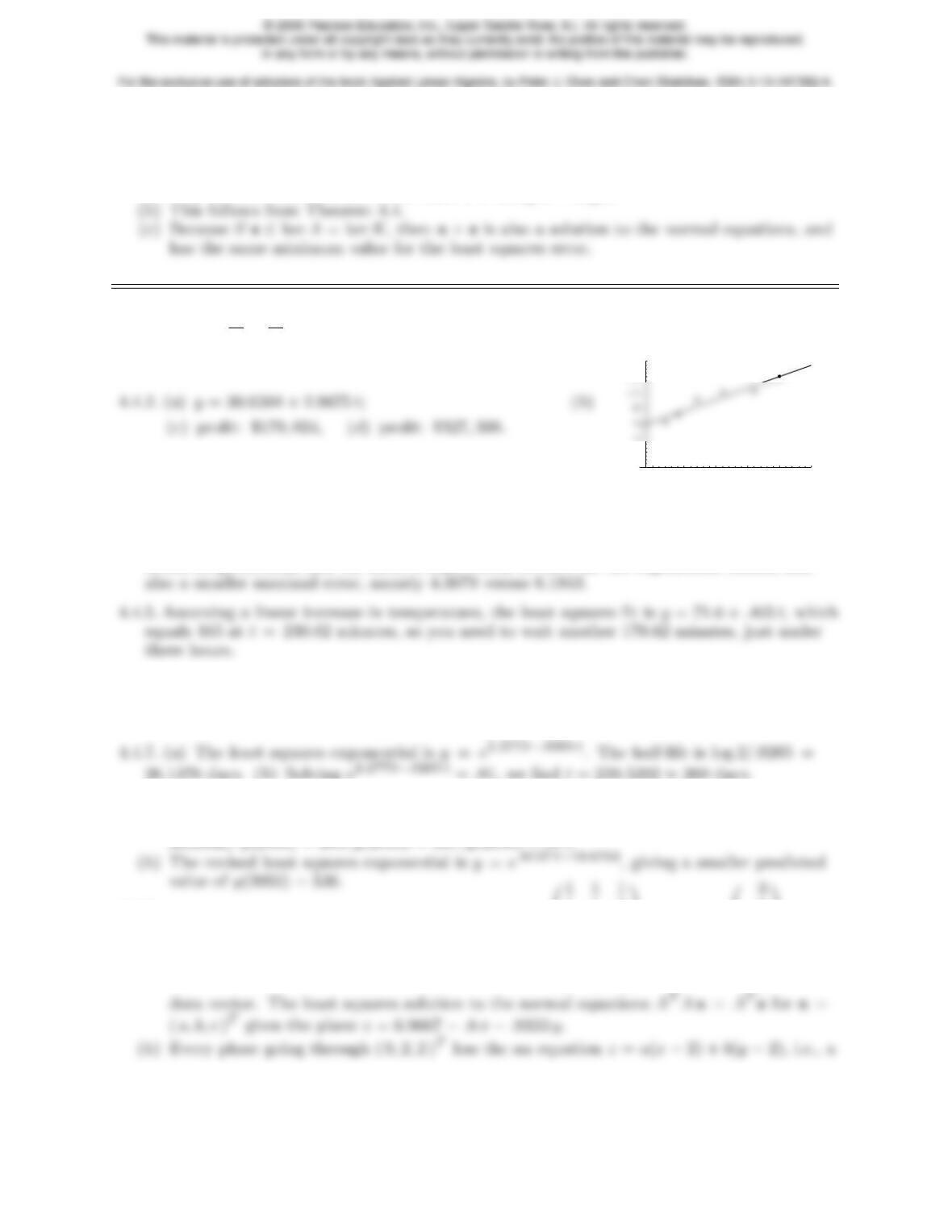
4.4.1. (a)y=12
7+12
7t= 1.7143 (1 + t); (b)y= 1.9−1.1t; (c)y=−1.4 + 1.9t.
10 15 20 25 30 35
20
120
140
4.4.3. (a)y= 3.9227 t−7717.7; (b) $147,359 and $166,973.
♥4.4.4. (a)y= 2.2774t−4375; (b) 179.75 and 191.14; (c)y=e.0183 t−31.3571, with esti-
mates 189.79 and 207.98. (d) The linear model has a smaller the least squares error be-
tween its predictions and the data, 6.4422 versus 10.4470 for the exponential model, and
4.4.6.
(a) The least squares exponential is y=e4.6051−.1903 tand, at t= 10, y= 14.9059.
(b) Solving e4.6051−.1903 t=.01, we find t= 48.3897 ≈49 days.
26.1376 days. (b) Solving e2.2773−.0265 t=.01, we find t= 259.5292 ≈260 days.
4.4.8.
(a) The least squares exponential is y=e.0132 t−20.6443, giving the population values (in
millions) y(2000) = 296, y(2010) = 337, y(2050) = 571.
4.4.9.
(a) The sample matrix for the functions 1, x, y is A=
B
B
B
B
B
B
B
@
1 1 2
1 2 1
1 2 2
1 3 2
1 3 4
C
C
C
C
C
C
C
A
, while z=
B
B
B
B
B
B
B
@
6
11
−2
0
3
C
C
C
C
C
C
C
A
is the
109
0
−1−1
1
♦4.4.10. For two data points t1=a, t2=b, we have
t2=1
2(a2+b2),while (t)2=1
4(a2+ 2ab +b2),
♦4.4.11.
1
m
m
X
i= 1
(ti−t)2=1
m
m
X
i= 1
t2
i−2t
m
m
X
i= 1
ti+(t)2
m
m
X
i= 1
1 = t2−2 ( t)2+ ( t)2=t2−(t)2.
4.4.12.
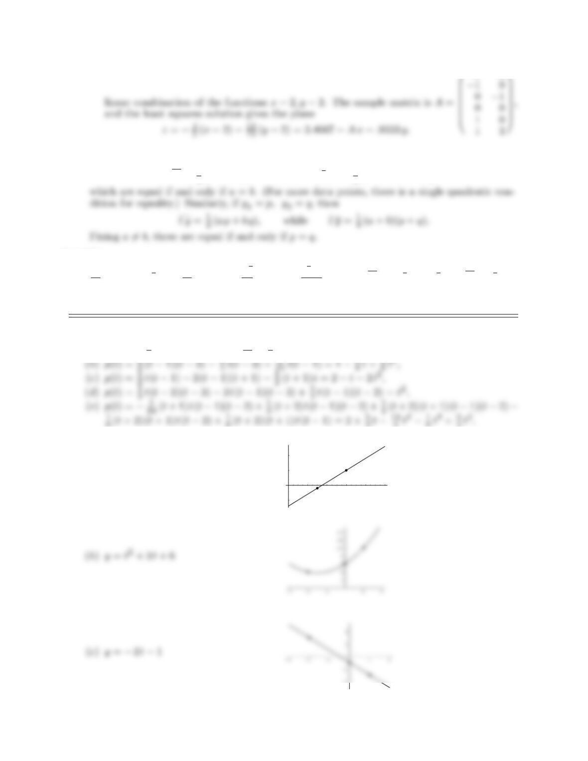
(a)p(t) = −1
5(t−2) + (t+ 3) = 17
5+4
5t,
4.4.13.
(a)y= 2t−7
246 8 10
-5
5
10
-4
110
© 2006 Pearson Education, Inc., Upper Saddle River, NJ. All rights reserved.
This material is protected under all copyright laws as they currently exist. No portion of this material may be reproduced,
in any form or by any means, without permission in writing from the publisher.
For the exclusive use of adopters of the book Applied Linear Algebra, by Peter J. Olver and Cheri Shakiban. ISBN 0-13-147382-4.
(d)y=−t3+ 2t2−1
-1.5 -1 -0.5 0.5 1 1.5 2 2.5
-3
-2
-1
1
2
3
4
5
-10
4.4.14.
(a)y=−4
3+ 4t.
(b)y= 2 + t2. The error is zero because the parabola interpolates the points exactly.
4.4.15.
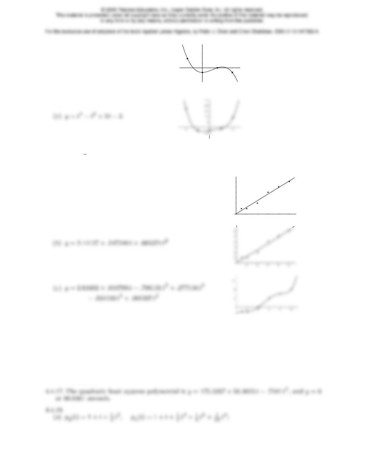
(a)y= 2.0384 + .6055 t
246 8 10
3
4
5
6
7
8
(d) The linear and quadratic models are practically identical, with almost the same least
squares errors: .729045 and .721432, respectively. The fifth order interpolating polyno-
mial, of course, has 0 least squares error since it goes exactly through the data points.
On the other hand, it has to twist so much to do this that it is highly unlikely to be
the correct theoretical model. Thus, one strongly suspects that this experimental data
comes from a linear model.
4.4.16. The quadratic least squares polynomial is y= 4480.5 + 6.05 t−1.825 t2, and y= 1500 at
42.1038 seconds.
111
(b) The maximal error for p2(t) over the interval [ 0,1 ] is .218282, while for p4(t) it is .0099485.
The Taylor polynomials do a much better job near t= 0, but become significantly worse
at larger values of t; the least squares approximants are better over the entire interval.
♥4.4.19. Note: In this solution tis measured in degrees! (Alternatively, one can set up and solve
the problem in radians.) The error is the L∞norm of the difference sin t−p(t) on the in-
terval 0 ≤t≤60.
4.4.20. (a) For equally spaced data points, the least squares line is y=.1617 + .9263 twith a
maximal error of .1617 on the interval 0 ≤t≤1. (b) The least squares quadratic poly-
nomial is y=.0444 + 1.8057 t−.8794 t2with a slightly better maximal error of .1002.
4.4.21. p(t)=.9409 t+.4566 t2−.7732 t3+.9330 t4. The graphs are very close over the interval
0≤t≤1; the maximum error is .005144 at t=.91916. The functions rapidly diverge above
1, with tan t→ ∞ as t→1
2π, whereas p(1
2π)=5.2882. The first graph is on the interval
4.4.22. The exact value is log10 e≈.434294.
(a)p2(t) = −.4259 + .48835 t−.06245 t2and p2(e)=.440126;
(b)p3(t) = −.4997 + .62365 t−.13625 t2+.0123 t3and p2(e)=.43585.
♦4.4.23.
(a)q(t) = α+β t +γ t2where
α=−y0t1t2(t2−t1)+y1t2t0(t0−t2)+y2t0t1(t1−t0)
(t1−t0)(t2−t1)(t0−t2),
112
♠4.4.24. When a < 2, the approximations are very good. At a= 2, a small amount of oscillation
is noticed at the two ends of the intervals. When a > 2, the approximations are worthless
for |x|>2. The graphs are for n+ 1 = 21 iteration points, with a= 1.5,2,2.5,3:
0.8
1
0.8
1
0.8
1
0.8
1
♠4.4.25. The conclusions are similar to those in Exercise 4.4.24, but here the critical value of ais
around 2.4. The graphs are for n+ 1 = 21 iteration points, with a= 2,2.5,3,4:
0.6
0.8
1
0.6
0.8
1
0.6
0.8
1
0.6
0.8
1
4.4.26. x∈ker Aif and only if p(t) vanishes at all the sample points: p(ti) = 0, i= 1, . . . , m.
4.4.27.
(a) For example, the the interpolating polynomial for the data (0,0),(1,1),(2,2) is the
straight line y=t.
(b) The Lagrange interpolating polynomials are zero at nof the sample points. But the
only polynomial of degree < n than vanishes at npoints is the zero polynomial, which
does not interpolate the final nonzero data value.
♦4.4.28.
(a) If p(xk)=a0+a1xk+a2x2
k+···+anxn
k= 0 for k= 1,…,n+ 1, then Va=0
♦4.4.29. This follows immediately from (4.51), since the determinant of a regular matrix is the
product of the pivots, i.e., the diagonal entries of U. Every factor ti−tjappears once
among the pivot entries.
113
♥4.4.31.
(a)f0(x)≈f(x+h)−f(x−h)
2h;
(b)f00(x)≈f(x+h)−2f(x) + f(x−h)
h2;
h4.
(e) For f(x) = exat x= 0, using single precision arithmetic, we obtain the approximations:
For h=.1: f0(x)≈1.00166750019844,
f00(x)≈1.00083361116072,
f0(x)≈.99640457071210,
For h=.0001: f0(x)≈1.00000000166730,
f00(x)≈1.00000001191154,
When f(x) = tan xat x= 0, using single precision arithmetic,
For h=.1: f0(x)≈1.00334672085451,
f00(x)≈3.505153914964787 ×10⁻¹⁶,
For h=.01: f0(x)≈1.00003333466672,
f00(x)≈ −2.470246229790973 ×10⁻¹⁵,
f0(x)≈.99993331466332,
For h=.001: f0(x)≈1.00000033333347,
f00(x)≈ −3.497202527569243 ×10⁻¹⁵,
f0(x)≈.99999933333147,
f0(x)≈.99999999999947,
115
For the exclusive use of adopters of the book Applied Linear Algebra, by Peter J. Olver and Cheri Shakiban. ISBN 0-13-147382-4.
In most cases, the accuracy improves as the step size gets smaller, but not always. In
particular, at the smallest step size, the approximation to the fourth derivative gets
♥4.4.32.
(a) Trapezoid Rule: Zb
af(x)dx ≈1
2(b−a)hf(x0) + f(x1)i.
(b) Simpson’s Rule: Zb
af(x)dx ≈1
6(b−a)hf(x0)+4f(x1)+f(x2)i.
4.4.33. The sample matrix is A=0
B
@
1 0
0 1
−1 0 1
C
A; the least squares solution to Ax=y=0
B
@
1
.5
.25 1
C
A
gives g(t) = 3
8cos π t +1
2sin π t.
4.4.34. g(t) = .9827 cosh t−1.0923 sinh t.
4.4.35. (a)g(t) = .538642 et−.004497 e2t, (b).735894.
(c) The maximal error is .745159 which occurs at t= 3.66351.
4.4.36.
(a) 5 points: g(t)=−4.4530 cos t+ 3.4146 sin t= 5.6115 cos(t−2.4874);
For the exclusive use of adopters of the book Applied Linear Algebra, by Peter J. Olver and Cheri Shakiban. ISBN 0-13-147382-4.
♥4.4.37.
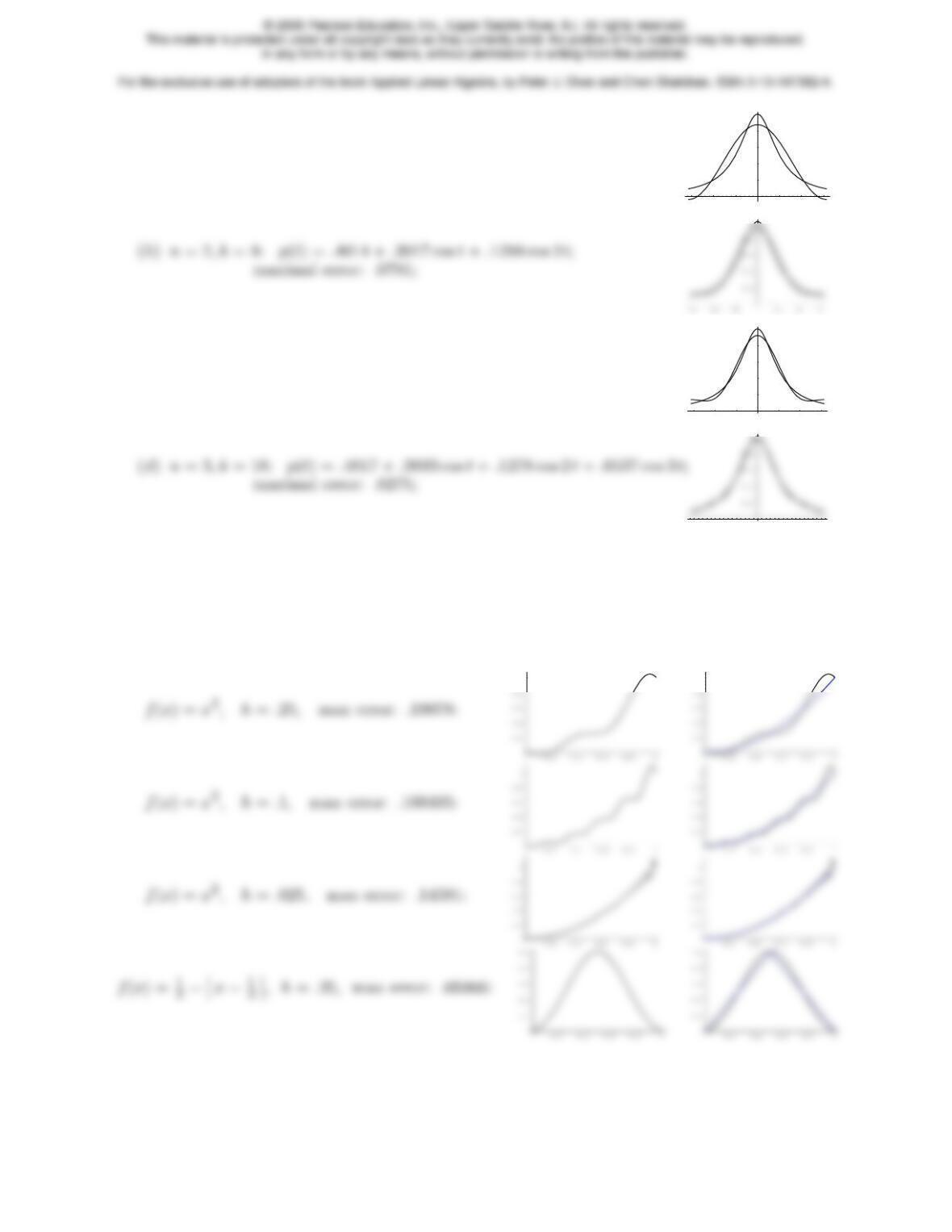
(a)n= 1, k = 4: p(t)=.4172 + .4540 cos t;
maximal error: .1722;
-3 -2 -1 1 2 3
0.2
0.4
0.6
0.8
1
(c)n= 2, k = 16: p(t) = .4017 + .389329 cos t+.1278 cos 2 t;
maximal error: .0812;
-3 -2 -1 1 2 3
0.2
0.4
0.6
0.8
1
-3 -2 -1 1 2 3
(e) Because then, due to periodicity of the trigonometric functions, the columns of the sam-
ple matrix would be linearly dependent.
♥4.4.38. Since Sk(xj) = (1, j =k,
0,otherwise., the same as the Lagrange polynomials, the coeffi-
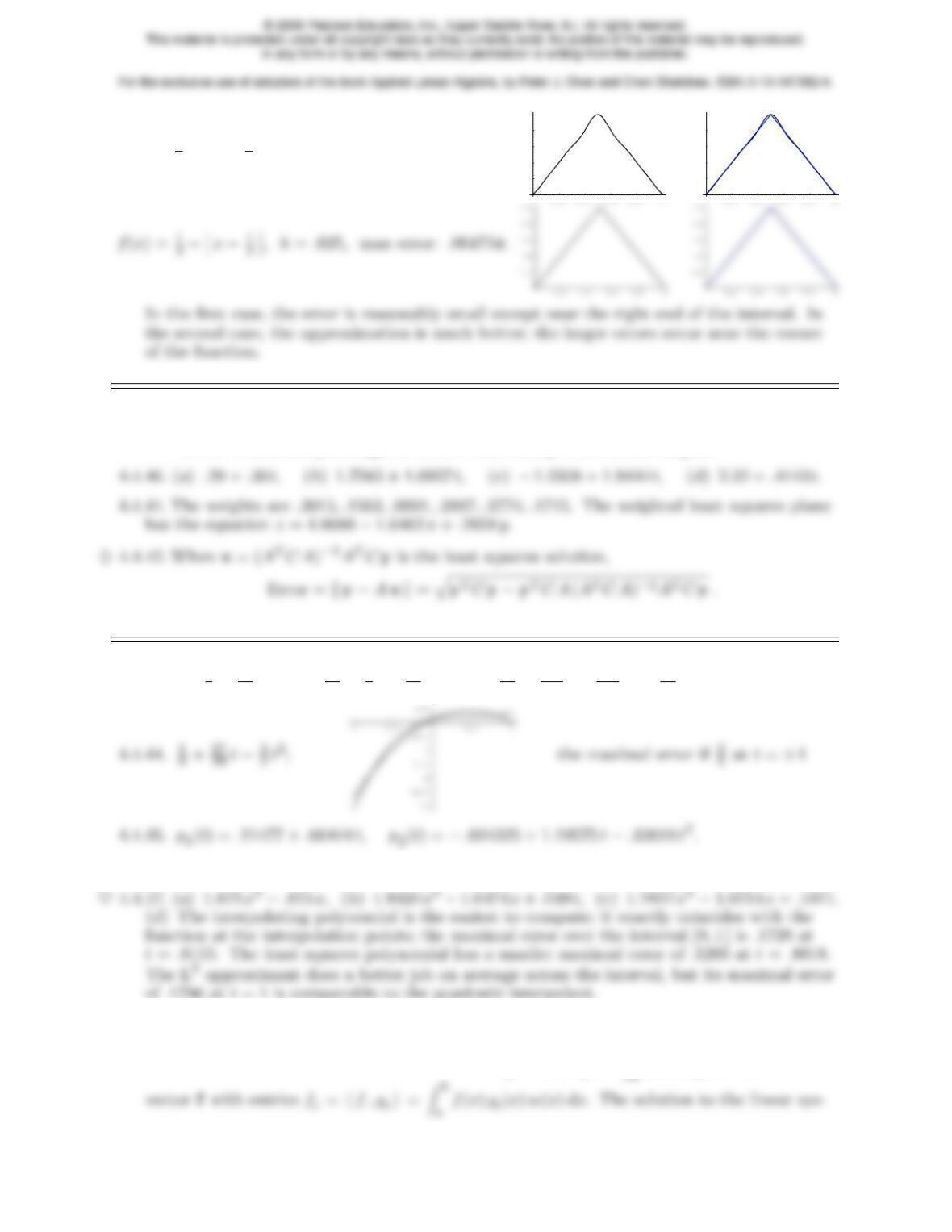
cients are cj=f(xj). For each function and step size, we plot the sinc interpolant S(x)
and a comparison with the graph of the function.
1
1
117
f(x) = 1
2−˛
˛
˛x−1
2˛
˛
˛,h=.1, max error: .01877:
0.2 0.4 0.6 0.8 1
0.1
0.2
0.3
0.4
0.5
0.2 0.4 0.6 0.8 1
0.1
0.2
0.3
0.4
0.5
4.4.39. (a)y=−.9231 + 3.7692t, (b) The same interpolating parabola y= 2 + t2.
Note: When interpolating, the error is zero irrespective of the weights.
4.4.43. (a)3
7+9
14 t; (b)9
28 +9
7t−9
14 t2; (c)24
91 +180
91 t−216
91 t2+15
13 t3.
4.4.46. 1.00005 + 0.99845 t+.51058 t2+ 0.13966 t3+.069481 t4.
4.4.48. g(x) = 2 sin x.
♦4.4.49. Form the n×nGram matrix with entries kij =hgi, gji=Zb
118
4.4.50.
(i)3
28 −15
14 t+25
14 t2≈.10714 −1.07143 t+ 1.78571 t2; maximal error: 5
28 =.178571 at t= 1;
(ii )2
7−25
14 t+50
21 t2≈.28571 −1.78571 t+ 2.38095 t2; maximal error: 2
7=.285714 at t= 0;
(iii ).0809 −.90361 t+ 1.61216 t2; maximal error: .210524 at t= 1. Case (i) is the best.
♥4.4.51.
∞
119