Chapter 15
15.1
2
2
1
1
..
. . .. ..
()
[2 ]
11
a
ia
i
ii
i
nxx nxxxx
aa
15.2
2
11
22
11 11
2
2
22
11
..
.. ..
.. ..
..
()
2
2
an
ij
ij
an an
ij ij
ij ij
an
ij
ij
SST x x
x x x nax
T naT
xT
na na
Chapter 15 227
15.3
22
.
11 11
.. .. .
() [()(]
ii
nn
aa
ij i ij i
ij ij
xx xx xx
SST is such that
2
SST
σ
is value of random variable having
2
χ
distribution with
1
11
a
i
i
nN
degrees of freedom. For each i,
2
2
1
.
1()
i
n
ij i
j
xx
σ
is value of random variable
15.4
2
11
22
11 11 11
..
.. ..
()
2.
i
iii
n
a
ij
ij
nnn
aaa
ij ij
ij ij ij
SST x x
xx x x
228 Mathematical Statistics, 8E
15.5
22
11 2 2
... ...
() ( ) ( )SS Tr n x x n x x
11 2 2
12
..
..
nx nx
xnn
12
12
2222
11 2 2 1 1 2 2
11
2
12
..
( ) ( )(1)(1)
(2)
nn
jj
jj
SSE x x x x n s n s
nn sp
15.6
2
11
[( )]
i
n
a
ij i i
ij
ux
μ
αλα
11
2 [ ( )]( 1) 0
i
n
a
ij i
ij
ux
μα
μ
Chapter 15 229
15.7
2
11
..
()
an
ij
ij
xx
2
11
22
11
... . .. .. ..
... . ..
[( )( )( )]
() ( )
an
ijijij
ij
an
ij
ij
xx x x xxx x
nxx axx
15.8
ij i j
μ
μα β
11 11 11 11
11
()
an an an an
ij i j
ij ij ij ij
na na
μ
αβ μ α β
230 Mathematical Statistics, 8E
15.9
222
11
... . .....
() [2 ]
11
nn
jjj
ji
aa
xx x xxx
nn
15.10
2
1
22
11 1
2
2
2
1
22
1
...
. . .. ..
.
.. .. ..
...
()
2
2()
11
( ) QED
n
j
j
nn n
jj
jj j
n
j
j
n
j
j
SSB a x x
ax axxax
T
a ax nx nax
k
TT
ana
Chapter 15 231
15.12 Dropping the indexes of summation for simplicity, we have
15.13 By Theorem 15.5,
22222
…
111
.. … .. .. ..
()
aaa
iii
iii
SSA rb x x rb x ax rb x rbax
Now,
.. …
.. …
and
i
i
TT
xx
rb rba
Thus,
2
a
232 Mathematical Statistics, 8E
15.14 First we write the identity
() () () ()
.. .. .. . .. .. . . ..
()()( )( 2)
ij k i j k ij k i j k
xxxxxxxxxxxxx
Then we square each side of the equation and sum each term on i and j from 1 to n.
ij
15.15 The left-hand side of the identity in Exercise 15.14 is the total sum of squares, SST; the terms
on the right-hand side are, respectively, the row sum of squares, SSR, the column sum of
squares, SSC, the treatment sum of squares, SS(Tr) and the error sum of squares, SSE. Thus, we
can write the following analysis-of-variance table for the Latin square of size n.
Source of
Variation
Degrees of
Freedom
Sum of
Squares
Mean
Square
F
Rows
1n
SSR
/
(1)SSR n
/MSR MSE
/
/
111
kji
15.16
12 3
2
.......
3, 8, 456.8, 473.4, 547.6, 1477.8,
and 91,939.96
anT T T T
x
Chapter 15 233
15.17
1234
2
…...
4, 5, 70, 75, 79, 69, 293,
and 4407
anTTTTT
x
15.18
2
1. 2. 3. ..
3, 6, 135, 120, 78, 333, 6507anT T T T x
2
1
6507 (333) 6507 6160.5 346.5 (d.f. 17)
18
SST
15.19
1234 1. 2.
3. 4. ..
4, 8, 8, 6, 9, 31, 574, 547,
449, 584, 2154
annnnN T T
TTT
2
41,386 37,491 33,683 38,064 150,624x
234 Mathematical Statistics, 8E
15.20
123 1 2 3
...
3, 4, 2, 3, 9, 1908, 990, 1445,
an n n N T T T
15.21
123 1.2.
2
3. ..
3, 400, 500, 400, 1300, 81, 72,
43, 196, 840
an n n N T T
TT x
15.22 1 0 1
A 12 23 89
124
B 8 12 62
82
12
3
1. 2. 3.
3, 124, 82
170, 376
77, 54, 98
kn n
nN
TTT
Chapter 15 235
15.23
123 1
234
....
. . . …
3, 4, T 197.4, 185.9 206.0, T 137.6,
165.5, 157.6, 128.6, 589.3
an T T
TTTT
2
9,888.3 8,732.45 10.697.8 29,318.55x
15.24
1234 1
23
…..
. . …
4, 3, T 8.8, 8.8, 9.7, =10.3, T 13.2,
11.4, 13.0, 37.16
an T T T
TTT
2
26.16 25.9 31.45 35.55 119.06x
15.25
123 4 5
1234
... ..
…....
5, 4, T 83.1, 103, 94.5, T 95.2, 85,
115.8, 112.1, 114, 118.9, 460.8
an T T T
TTTTT
2
17.28.59 2655.48 2241.47 2277.22 1810.42 10,713.18x
236 Mathematical Statistics, 8E
15.26 Teacher Lawyer Doctor
East I R D
I = independent
15.27 Summing the observations in each replicate, we have
12
.. ..
589.3, 595.8.TT
Summing over the two replicates, we obtain the following two-way table:
Fuels
Launchers 1 2 3 4 Totals
X 92.0 113.5 104.8 86.0 396.3
Y 92.3 103.1 101.5 78.4 375.3
Z 91.5 114.8 111.5 95.7 413.5
Totals 275.8 331.4 317.8 260.1 1,185.1
2
(1,185.1) 58,519.25
24
C
ANALYSIS OF VARIANCE
Source of
Variation
Degrees of
Freedom
Sum of
Squares
Mean
Square
F
Critical
0.01
F
Launchers 2 91.40 45.75 83.2 7.21
Fuels 3 570.83 190.28 346.0 6.22
Chapter 15 237
15.28 Summing the observations in each replicate, we have
12
.. ..
37.6, 39.0TT
. Summing over
the two replicates, we obtain the following two-way table:
Foods
Laboratories A B C Totals
1 6.9 5.1 5.7 17.7
2
(76.6) 244.48
24
C
(Total) 247.28 2.80
(Error) (Laboratories) (Foods)
SS C
SS SST SS SS
(Replicates) (Interaction) 0.31SS SS
ANALYSIS OF VARIANCE
Source of
Variation
Degrees of
Freedom
Sum of
Squares
Mean
Square
F
Critical
0.05
F
Laboratories 3 1.22 0.41 13.7 3.59
Foods 2 0.64 0.32 10.7 3.98
15.29 Summing the observations in each replicate, we have
12
.. ..
122.8, 122.7.TT
Summing over the two replicates, we obtain the following two-way table:
Bonders
Operators A B C D Totals
1 22.4 21.5 22.4 20.1 86.4
238 Mathematical Statistics, 8E
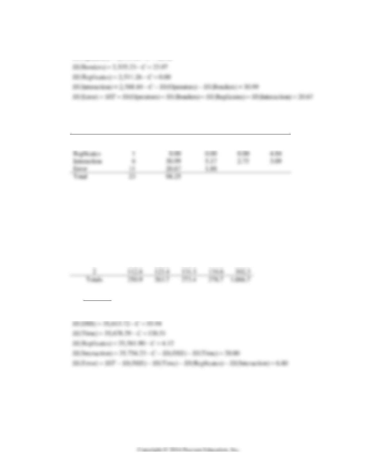
(Total) 2,609.51 98.25
(Operators) 2,533.88 22.62
SS C
SS C
ANALYSIS OF VARIANCE
Source of
Variation
Degrees of
Freedom
Sum of
Squares
Mean
Square
F
Critical
0.05
F
Operators 2 22.62 11.31 6.02 3.98
Bonders 3 23.97 7.99 4.25 3.59
Thus, the Operators and Bonders means are significantly different at the 0.05 level of
significance.
15.30 Summing the observations in each replicate, we have
12
.. ..
266.6, 267.0,TT
34
.. ..
262.5, 270.6.TT
Summing over the two replicates, we obtain the following two-way table:
DSS
Time 0 50 100 150 Totals
1 138.1 140.3 141.9 144.1 564.4
2
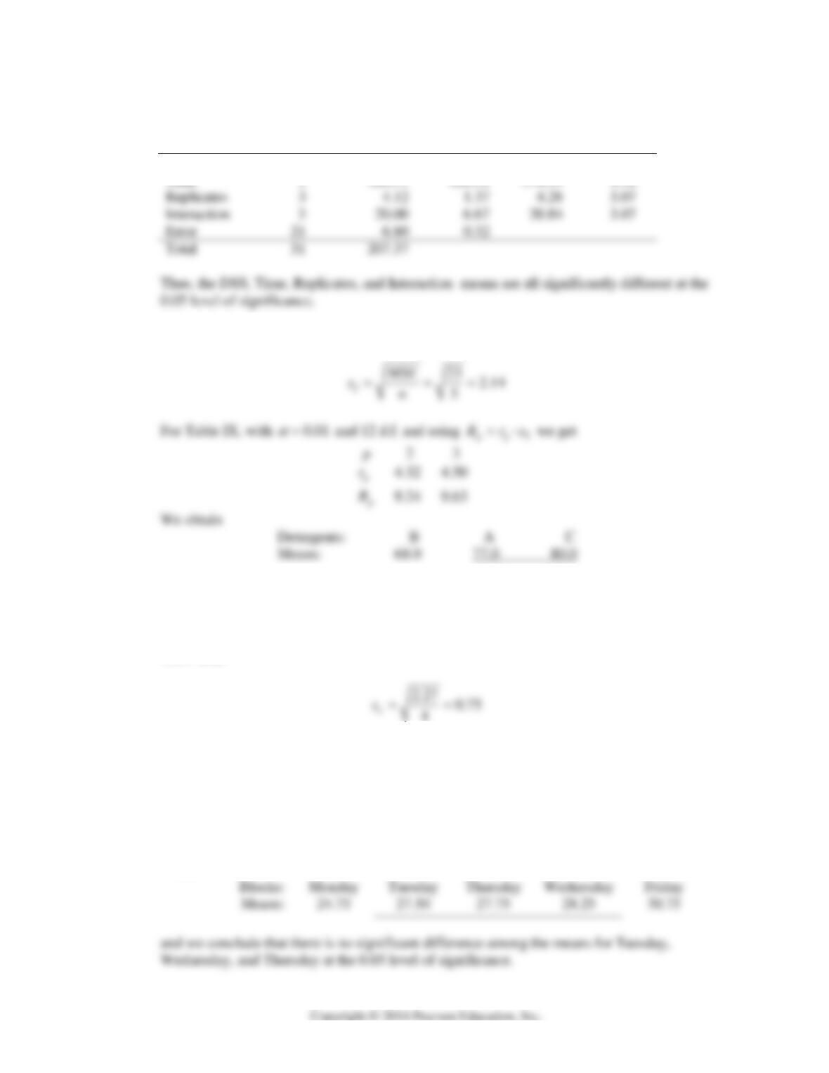
(1,066.7) 35,557.78
24
C
(Total) 35,765.15 207.37
SS C
Chapter 15 239
ANALYSIS OF VARIANCE
Source of
Variation
Degrees of
Freedom
Sum of
Squares
Mean
Square
F
Critical
0.05
F
DSS Level 3 55.94 18.65 58.28 3.07
Time 1 120.51 120.51 376.59 4.32
15.31 The three detergent means are: A: 77.0 B: 68.0 C: 80.0
R
R
and we conclude that detergents A and C do not give rise to significantly different means at the
0.01 level so significance.
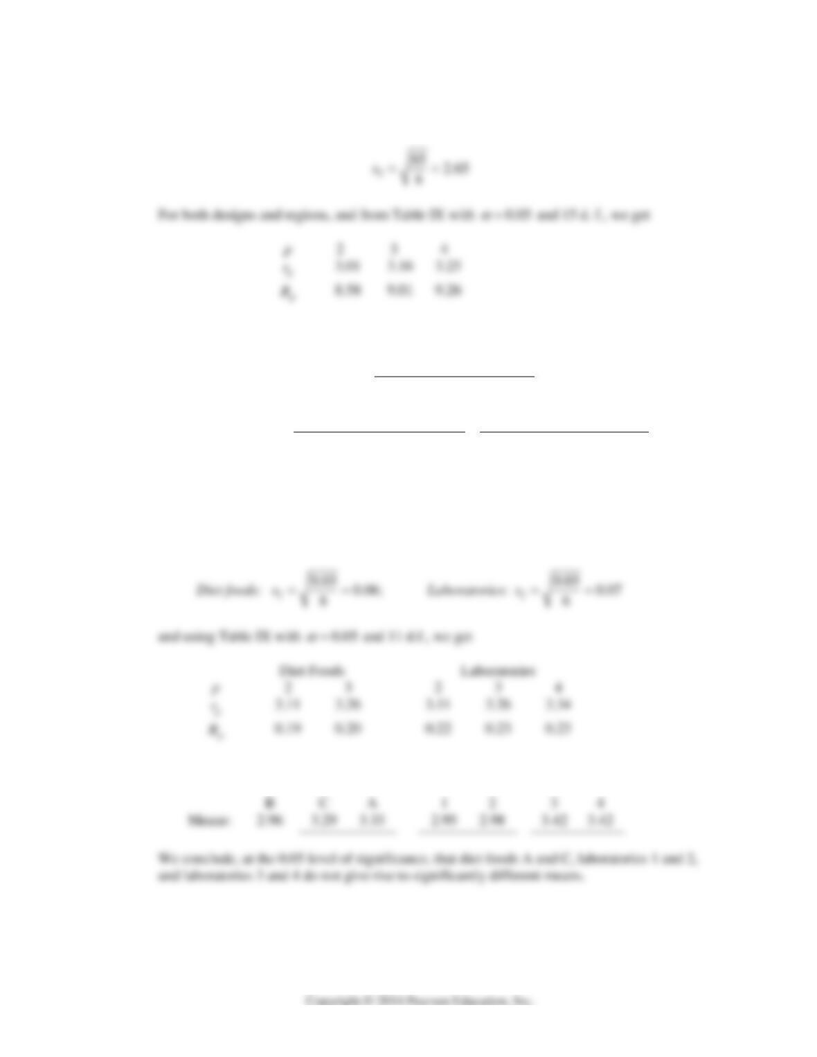
15.32 The five block means are: 24.75, 27.50, 28.25, 27.75, and 30.75. Proceeding as in Exercise
15.31 with
we obtain from Table IX, with
0.05
α
and 12 d.f.
p 2 3 4 5
p
r
3.08 3.23 3.31 3.37
p
R
2.31 2.42 2.48 2.53
Thus,
240 Mathematical Statistics, 8E
15.33 The four compressor-design means are: 46.50, 22.63, 61.25, and 48.00. The four region means
are: 52.88, 40.50, 52.88, and 32.13. With
Thus,
Designs: B A D C
Means: 22.63 46.50 48.00 61.25
Regions: Southwest Southeast Northwest Northeast
Means: 32.13 40.50 52.88 52.88
We conclude, at the 0.05 level of significance, that designs A and D do not give rise to
significantly different means and that the same is true for the Southwest and Southeast and for
the Northwest and northeast regions.
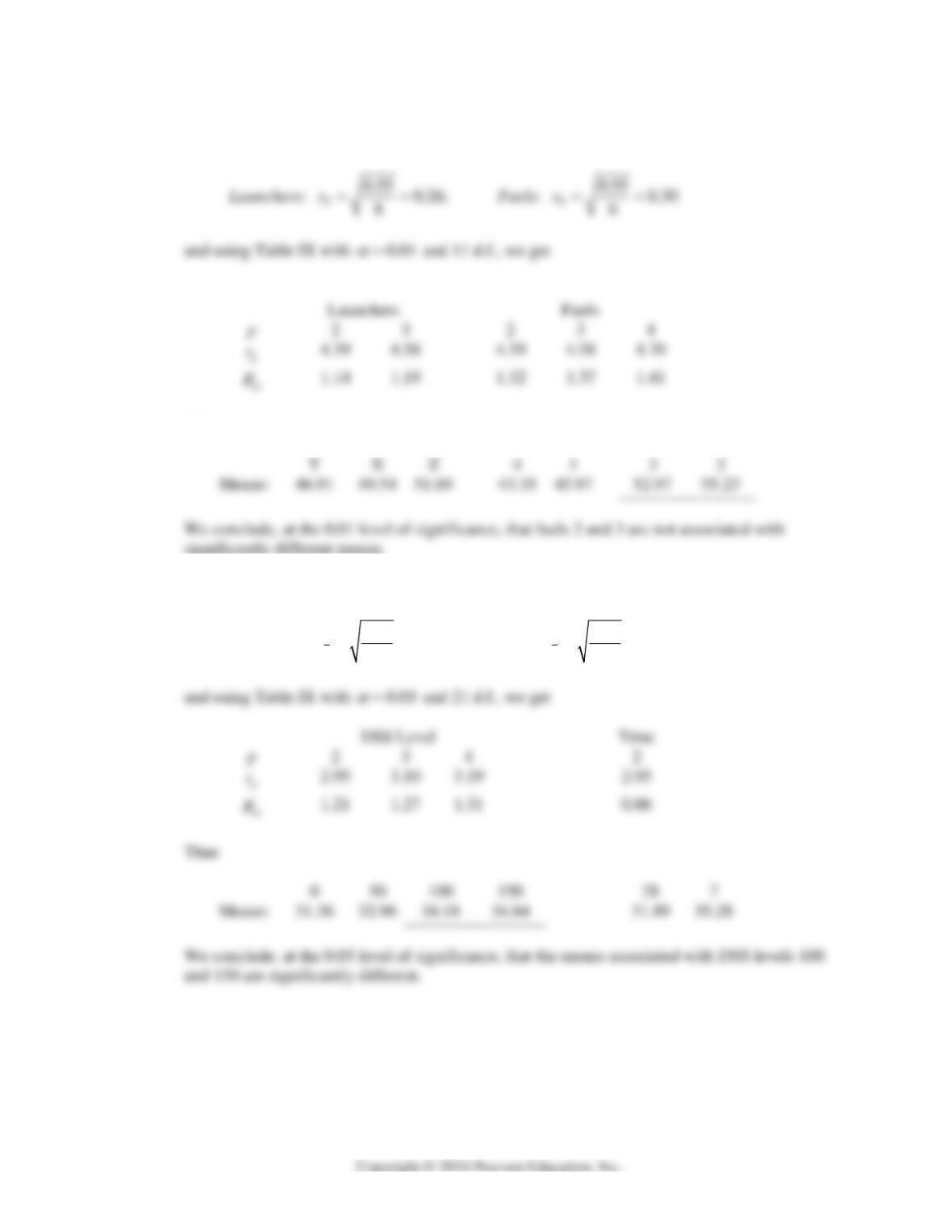
15.34 The three diet-food means are: 3.33, 2.96, and 3.29. The four laboratory means are 2.95, 2.98,
3.42, and 3.42. With
Thus
Chapter 15 241
15.35 The three launcher means are: 49.54, 46.91, and 51.69. The four fuel means are: 45.97, 55.23,
52.97, and 43.35. With
Thus
15.36 The DSS means are: 31.36, 32.96, 34.18, and 34.84. With
DSS Level:
1.37 0.41
8
x
s
; Time:
1.37 0.29
16
x
s
242 Mathematical Statistics, 8E
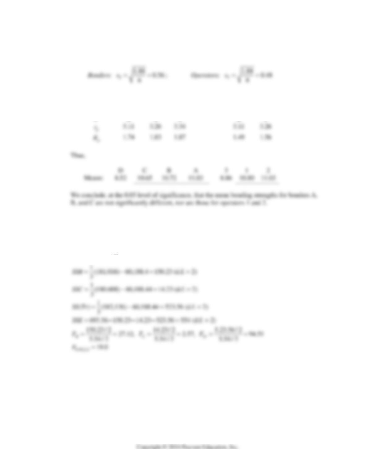
15.37 The Bonder means are: 11.03, 10.72, 10.65, and 8.52. The Operator means are: 10.80, 11.03,
and 8.85. With
And using Table IX with
0.05
α
and 11 d.f., we get
Bonders Operators
15.38
123 12
3
…..
....
3, T 230, 260, 246, T 240, 248,
248, 244, 274, 218, 736
ABC
mTT T
TTTTT
2
17,782 22,662, 20,438 60,882x
2
1
60,882 (736) 60,882 – 60,188.44 693.56 (d.f.= 8)
9
SST
(a)
Tr
F
(for instructor) = 94.5 is significant
(b)
C
F
= 2.57 (for ethnic background) is not significant
(c)
R
F
= 27.12 (for professional interest) is significant
Chapter 15 243
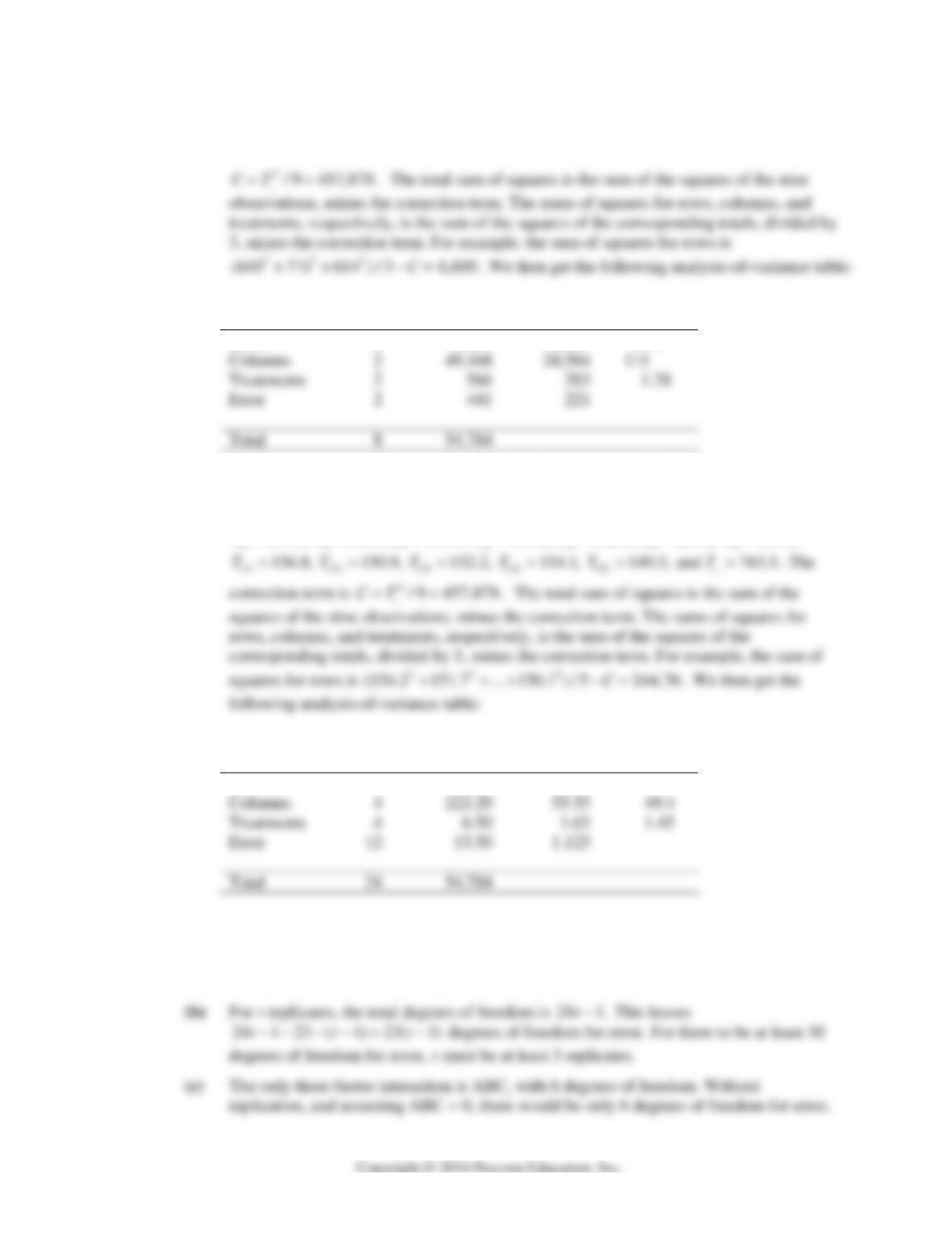
15.39 (a) First we calculate the following totals:
123
.. . . .
2,030, 645, 771, 614TTTT
,
12 3(1)(2)(3)
...
913, 380, 680, 646, 704TTTT T T
. The correction term is
Source of
Variability
Degrees of
Freedom
Sum of
Squares
Mean
Square
f
Rows 2 4,609 2,305 10.4
(b) No. With only 2 degrees of freedom for error, the f-tests have very little power.
15.40 (a) First we calculate the following totals:
123
.….
763.5, 154.2, 151.7, 143.2TTT T
154.3, =150.1, 161.4, 164.8, 152.1, 124.1, 161.1,TTTTTTT
Source of
Variability
Degrees of
Freedom
Sum of
Squares
Mean
Square
f
Rows 4 2.56 0.64 <1
15.41 (a) Factor Level 1 Level 2 Level 3 Level 4
A 1 2
B 1 2 3
C 1 2 3 4
244 Mathematical Statistics, 8E
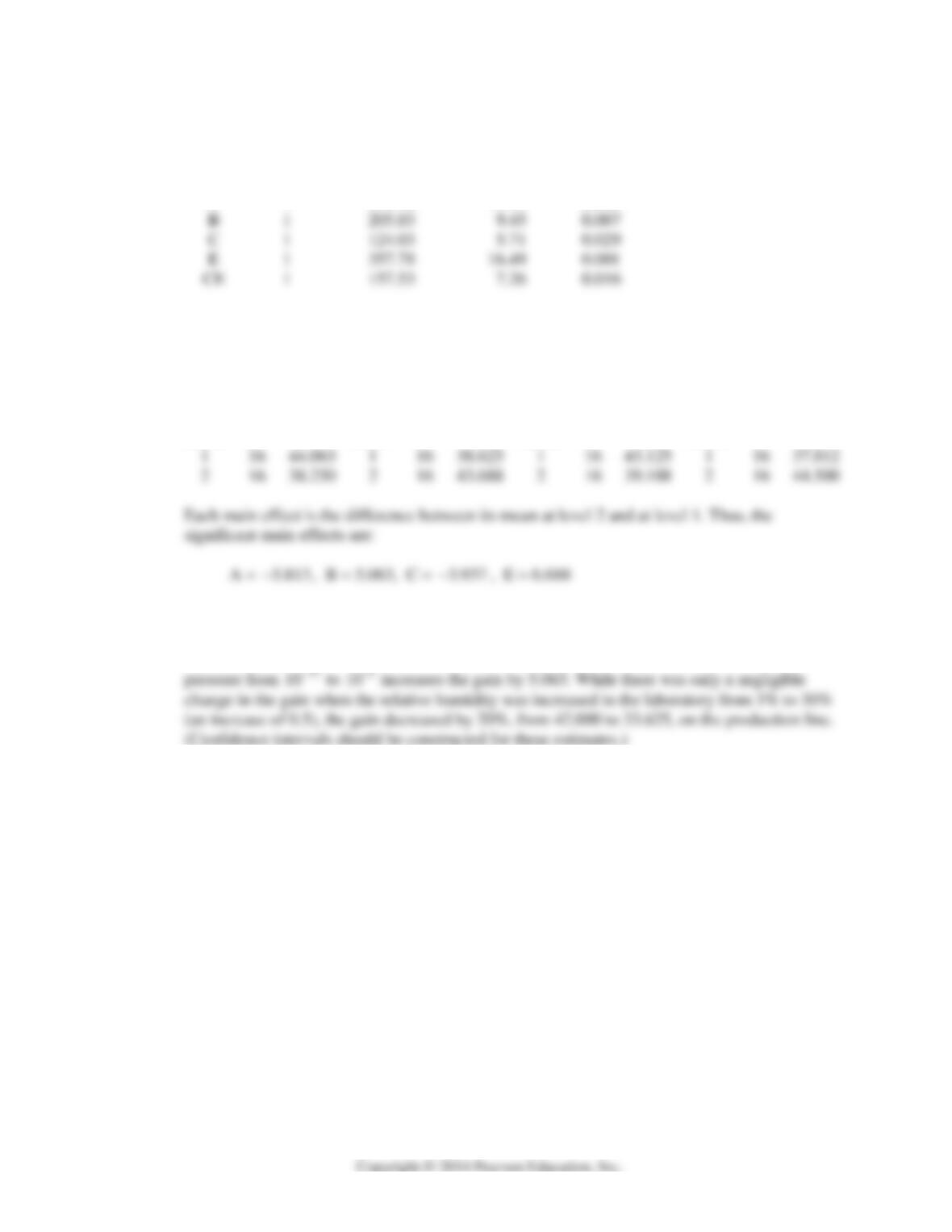
15.42 The analysis of variance shows the following significant effects (effects having P-values less
than or equal to 0.05).
Effect df Mean Square f P
A 1 270.28 12.45 0.003
15.43 There are 16 three-factor and higher-order interactions. If it is assumed that they do not exist,
there will be 16 degrees for freedom for error.
15.44 MINITAB software provides a table of means for the main effects. Here are the means for the
significant main effects.
Level N A Level N B Level N C Level N E
15.45. No. The effects C and E interact with each other.
15.47 Increasing temperature from 68° to 74°F decreases the gain by 5.813. Increasing the partial