Chapter 14 213
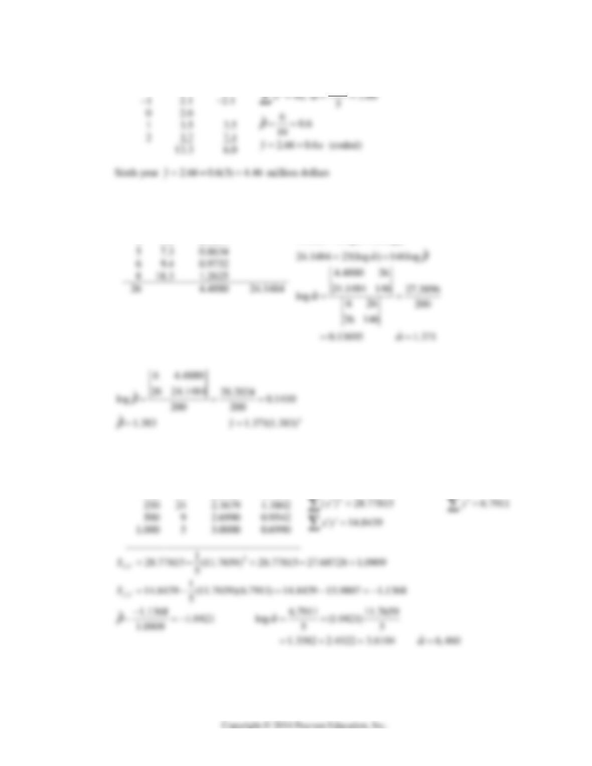
14.48
x
y
xy
2
1.4
2.8
2
13.3
14.49
x
y
‘log
yx
xy
1 2.0 0.3010
2 2.4 0.3802
4 5.1 0.7077
2
146
x
ˆ
ˆ
4.4880 6log 26log
a
β
14.50
log
xx
log
yy
x
y
x
y
50 108 1.6990 2.0334
100 53 2.0000 1.7243
n = 5
11.7659
x
214 Mathematical Statistics, 8E
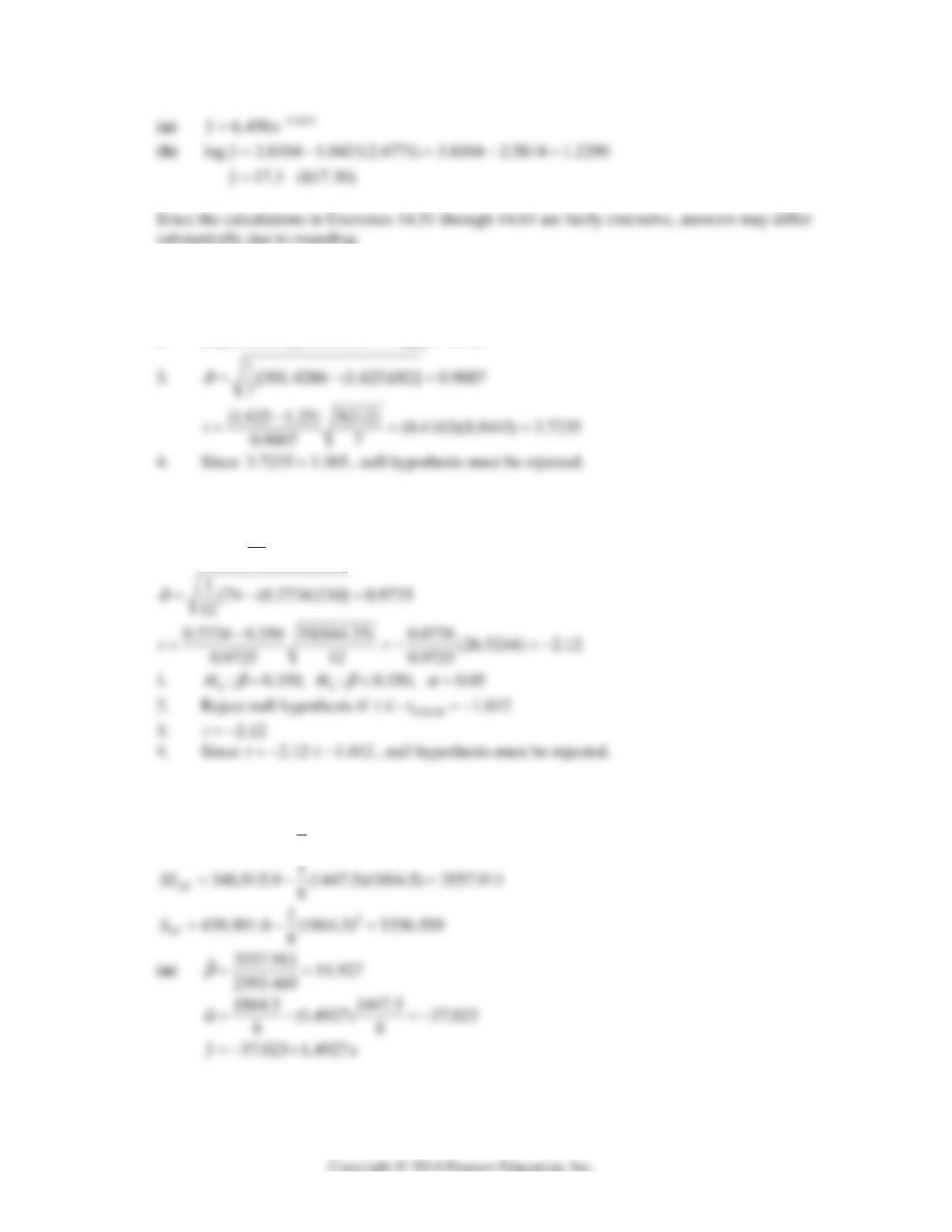
14.51
ˆ
7, 1.625, 112, 182, 301.4286
xx xy yy
n SSS
β
1.
01
: 1.25, : 1.25, 0.01
HH
β
βα
2. Reject null hypothesis if
3.365
tt
14.52
ˆ
12, 0.2724, 844.25, 230
xx xy
nSS
β
2
1
1802 (144) 1802 1728 74
12
yy
S
from Ex 14.18
β
14.53
22
8, 1447.5, 264,290.5, 1864.5, 439,901.6,
nx x y y
2
1
264,290.5 (1447.5) 2383.469
8
XX
SS
Chapter 14 215
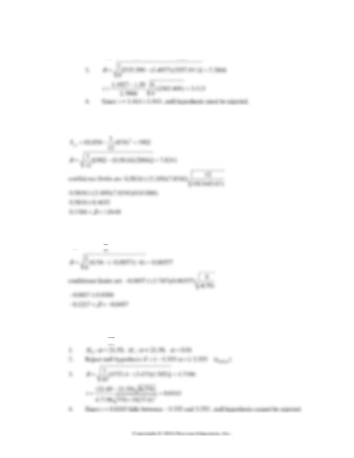
(b) 1.
01
:1.30, :1.30, 0.05
HH
β
βα
2. Reject null hypothesis if
0.05,6
1.943
tt
14.54
12, 3445.67, 2004
xx xy
nS S
ˆ0.5816
β
from Ex. 14.43
14.55
ˆ
6, 0.0857, 70, 6
xx xy
nSS
β
2
1
10.68 (7.8) 0.54
yy
S
14.56
ˆ
ˆ
10, 376, 1305, 21.69, 3.471
xx xy
nS S
αβ
2
1
36,562 (564) 4752.4
yy
S
216 Mathematical Statistics, 8E
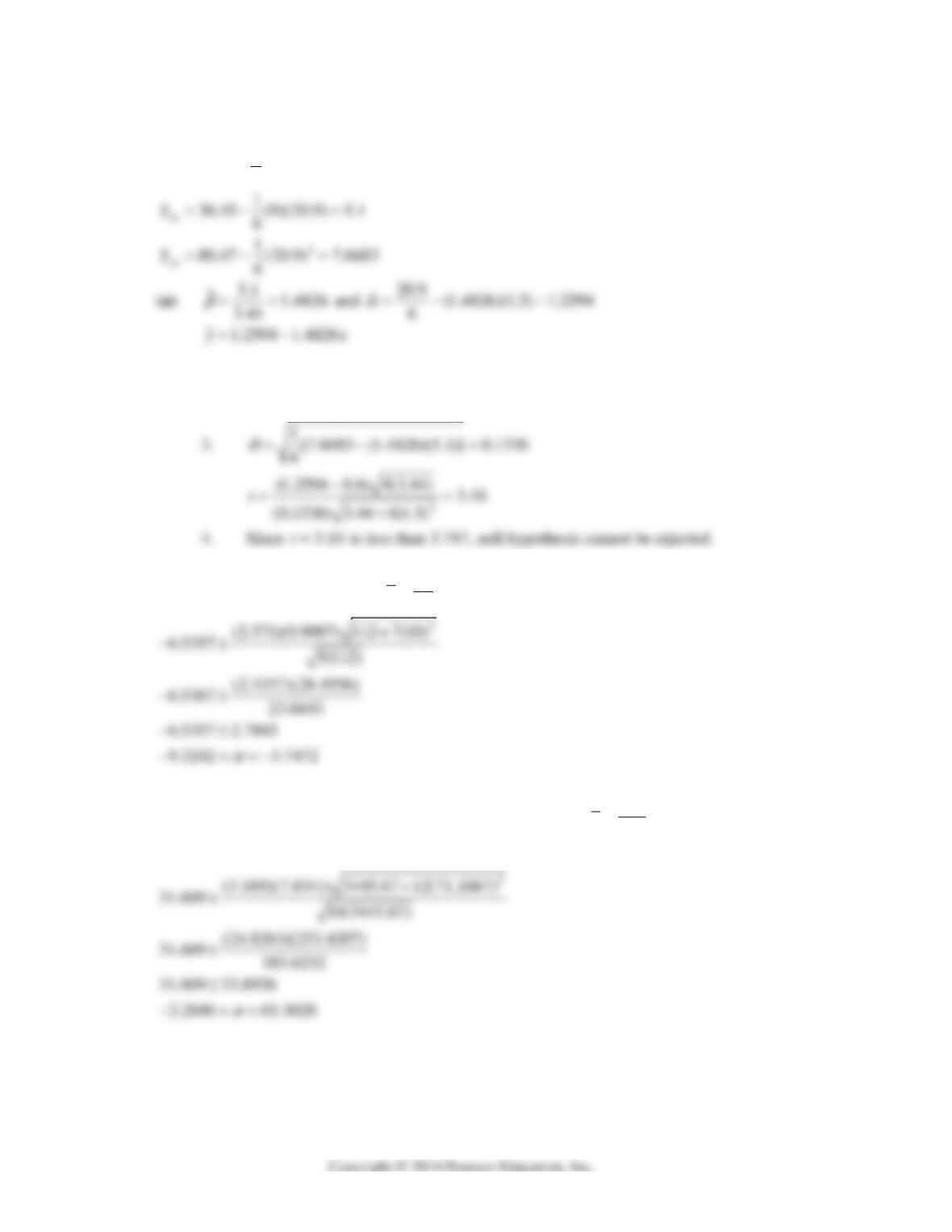
14.57
22
6, 9, 16.94, 20.9, 80.47, 36.45
nxx y y xy
2
1
16.94 (9) 3.44
6
xx
S
(b) 1.
01
: 0.08, : 0.08, 0.01
HH
ααα
2. Reject null hypothesis if
0.01,4
3.747
tt
14.58
0.025,5
70
ˆˆ
7, 6.5357, 112, 10, 0.9007, 2.571
7
xx
nSx t
ασ
14.59
0.005,10
854
ˆ
ˆˆ
12, 31.609, 0.5816, S 3445.67, 7.8341, 71.1667,
12
3.169
xx
nx
t
αβ σ
Chapter 14 217
14.60 (a)
3
10(14 10)
1376
70.284 (2.306)(4.720) 8
(b)
70.284 (3.8482) 11.4255
70.284 13.0075
Limits of prediction are 57.2765 and 83.2915
14.61
0 0.005,5 ˆ
7, 112, 10, 9, 4.032, 0.9007
xx
nS x x t
σ
,
0
ˆ6.5357 1.625(9) 8.0893
y
14.62
0
ˆ6.537 1.625 20 25.963
y
(a) The confidence limits are
2
7(20 10)
4.032 0.9007 1 112
25.963 or 25.963 4.373
5
14.63 (a) Using MINITAB
MTB> Regress C2 on 1 C1
The regression equation is
C2 = 2.20 + 13.3 C1
218 Mathematical Statistics, 8E
The 99% confidence limits for
β
are
/2, 2
ˆˆ:
(2)
n
xx
n
tnS
α
βσ
numerically,
10
13.27 (3.355)(3.38) (8)(50.70)
where
0.005,8 3.355
t
Table IV) and
β
14.64 Using MINITAB
MTB> Regress C2 1 C1
The regression equation is
C2 = 1.09 + 0.0131 C1
(b) We calculate:
2
340 15,500 573.10
xx xy
2
13.16 21.9072
yy
β
Chapter 14 219
14.65
22
20, 688, 24,282, 703, 25,555, 24,582
nx x y y xy
2
1
24,282 (688) 24,282 23,677.2 614.8
20
xx
S
2
1
25,555 (703) 25,555 24,710.45 844.55
yy
S
14.66
2(1.96)/ 17 0.951
0.951 0.951
1.553 0.447 1.553 0.447
1.553 0.447 1.553 0.447
ee
ee
ρ
14.67
22
33, 2550, 238,960, 861, 25,313, 74,476
nx x y y xy
238,960 197.045.45 41,914.55
xx
S
25,313 22,464.27 2,848.73
yy
S
74,476 66,531.82 7,944.18
xy
S
220 Mathematical Statistics, 8E
14.68
0.94 0.94
0.94 0.94
1.727 (0.273) 1.727 (0.273)
1.727 (0.273) 1.727 (0.273)
ee
ee
ρ
14.69
2
0.976 8
12.306
3.471 1 0.976
β
14.70 x y
12 27
26 36
22
10, 167, 4755, 288, 11,374,
7112
nx x y y
xy
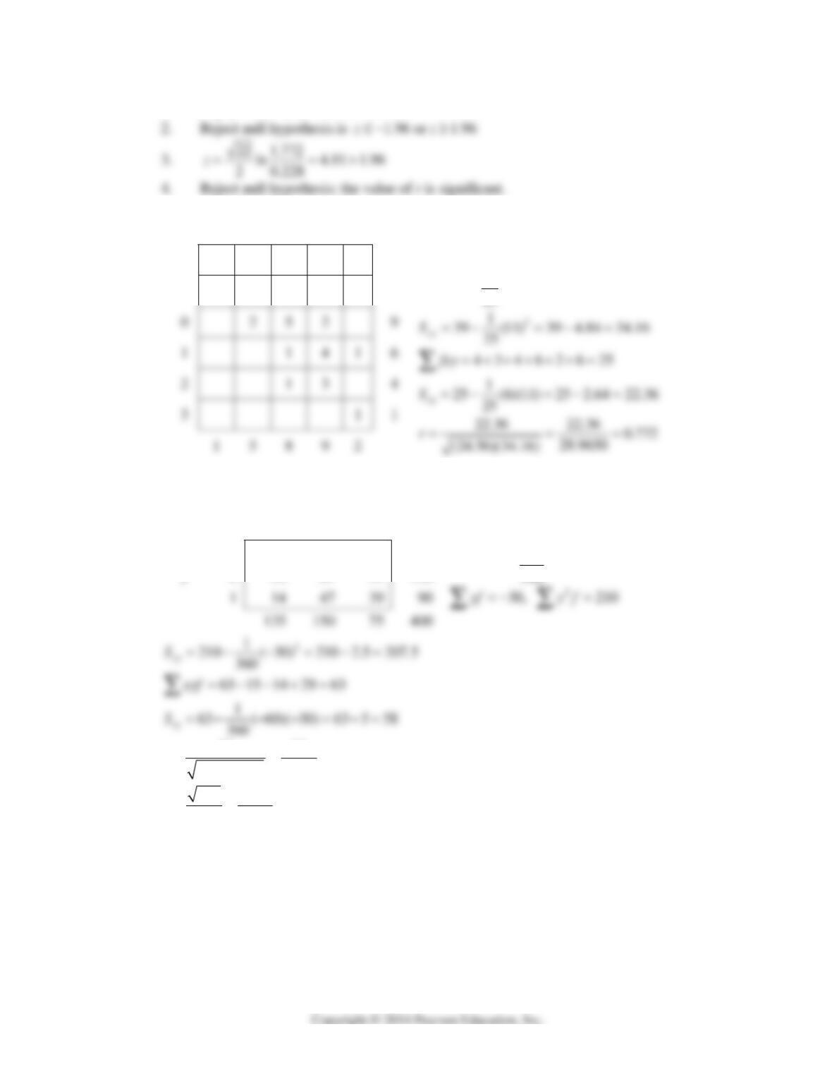
14.71 23 28 33 38 43
23 1 1
28 3 1 4
25
n
2
855 29,855
xf x f
29,855 29.241 614
xx
SS
2
880 =31,830
yf y f
Chapter 14 221
1.
01
:0; :0, 0.05HH
ρ
ρα
14.72 2 1 0 1 2
2 1 1
1 3 1 4
2
25, 6, 26nxx
2
11, 39yy
2
1
26 (6) 26 1.44 24.56
25
xx
S
14.73
x
1 0 1
1 63 42 15 120
y 0 58 61 31 150
2
60, 210xf x f
2
1
210 ( 60) 210 10 200
360
xx
S
58 58 0.285
203.7
200(207.5)
r
357 1.285
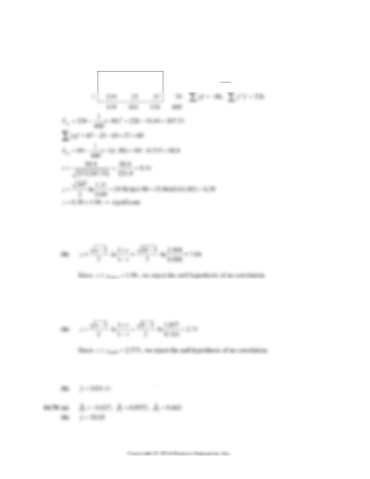
ln 9.447ln1.80 9.45(0.58779) 5.55
20.715
z
5.55 2.575z is significant
222 Mathematical Statistics, 8E
14.74
x
10 1
1 67 64 25 156
y 0 42 76 56 174
2
1, 237xf x f
2
1
237 ( 1) 237 0 237
400
xx
S
14.75 (a) Using the data of Exercise 14.63 and MINITAB:
MTB> Correlate C1 C2
Correlation of C1 and C2 = 0.994
0.02,5
14.76 (a) Using the data of Exercise 14.64 and MINITAB:
MTB> Correlate C1 C2
Correlation of C1 and C2 = 0.837
14.77 (a)
01 2
ˆˆ ˆ
14.56, 30.109, 12.16
ββ β
12
ˆ14.56 30.109 12.16yxx
Chapter 14 223
14.79 (a)
012
ˆˆˆ
124.57, 1.659, 1.439
βββ
(b) ˆ63.24y
14.82
0123
ˆˆˆˆ
2.33, 0.90, 1.27, 0.90
ββββ
12 3
ˆ2.33 0.90 1.27 0.90yxxx
14.83
01 2
ˆˆ ˆ
10.5, 2.0, 0.2
ββ β
2
10.5 2.0 0.2yxx
5.95y
β
14.87 0.16;t null hypothesis cannot be rejected
14.88
1
13.7 46.5
β
14.89 4.18t reject the null hypothesis
β
224 Mathematical Statistics, 8E
14.97 (a) Using MINITAB, we enter the values of y in C1 and
13
,xx
in C2,…C4.
MTB> Regress C1 on C2 C3 C4
14.99 (a) Using statistical software to fit the plane, we obtain
12
ˆ170 1.39 6.07yxx .
(b)
2
0.367R; the regression equation explains only 36.7% of the variability of y.
14.100(a) Using statistical software to fit the surface, we obtain
12 3
ˆ2,097 6.34 12.9 61.5yxxx .
(b) A computer generated normal-scores plot suggests little departure from normality.
14.101(b) Using statistical software, we find
2
122
ˆ86.9 0.904 0.508 2.06yxxx .
(c) The correlations among the independent variables are
22
12 12 22
0.142, 0.218, 0.421.
xx xx x x
rrr Although the correlation between
2
x and
14.102(b) Using statistical software, we find
12 312
ˆ11,024 98.2 170 2.70 185yxxxxx .
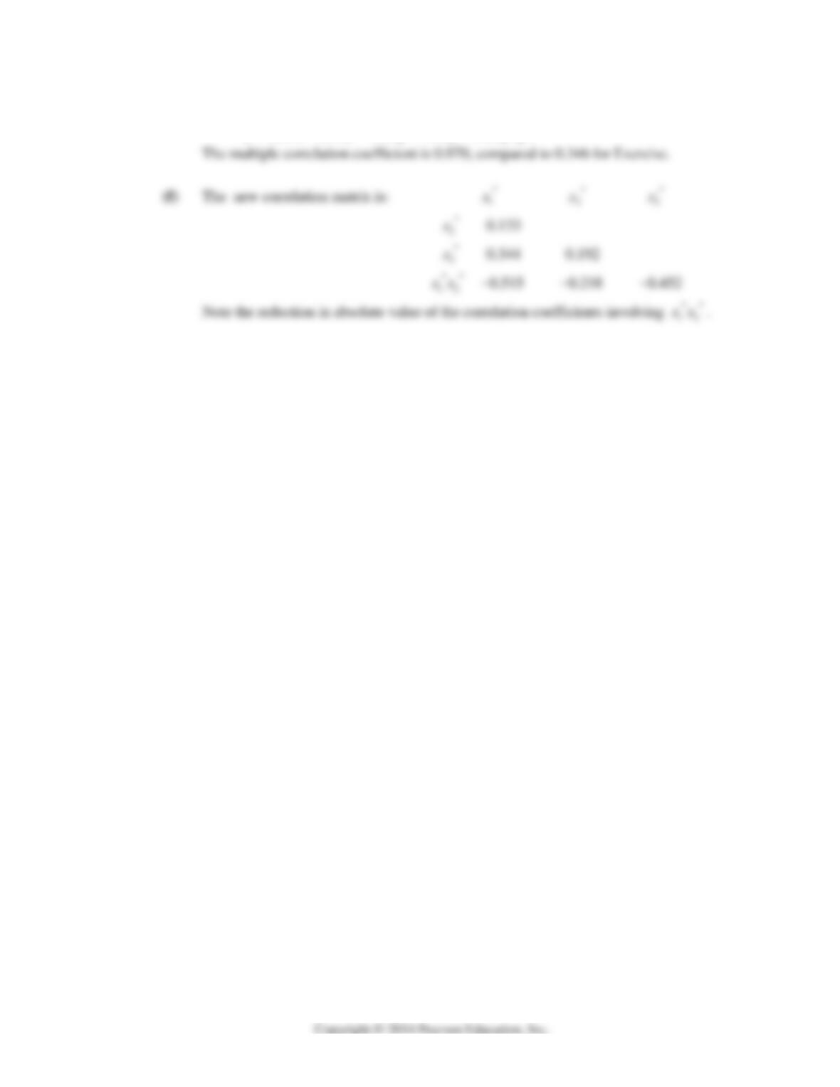
(c) The correlation matrix is:
1
x
2
x
3
x
Chapter 14 225
(e) The standardized regression equation is
12312
ˆ2,218 261 192 4.2 446yxxxxx
.