Chapter 14
14.1
(1 )
2
1
() (1 )
xy
hy xe dy y
14.2
1
0
223
() (2 3) 2
552
gx x ydy x
2(2 3 ) 23
5
() 3
23
2
22
52
xy xy
wyx
x
x
14.3
1
61
() 6 6(1 ), ( ) 6(1 ) 1
x
x
gx xdy x x wyx xx x
200 Mathematical Statistics, 8E
14.4
2
2
(, ) (1 )
x
fxy xxy
2
2
( ) 1
(1 )
x
g x dy u x xy du x dy
xxy
14.5
1
10 10 1 12 4
012
21 21 21 21 7
x
µ
0
51515 1639
0123
28 28 56 56 56 8
Y
µ
14.7
(, ) 2fxy
0
() 2 2
x
gx dx x
1
() 2 2(1 )
y
hy dx y
Chapter 14 201
2
(1)( 2)nmn
22
21 1 1 1
( ) , ( ) , ( ) , ( ) , ( )
33 2 6 4
Ex EY Ex EY ExY
14.8
0
() 24 12(1 )
gx x ydy x x
22
24 2
()
12 (1 ) (1 )
xy y
yx xx x
φ
13
2
22
0
22(1)2
(1 )
33
(1 ) (1 )
x
Yx
x
ydx x
xx
µ
202 Mathematical Statistics, 8E
14.9
( ) 0, ( ) 0 uncorrelatedEx ExY
1
() 0, ( ) , ( ) 0
3
Ex EY ExY
12
0 uncorrelated
σ
() 2, 0 1
y
hy dx y y
14.10
22
var( ) ( ) [ ( )]Yx EY x EYx
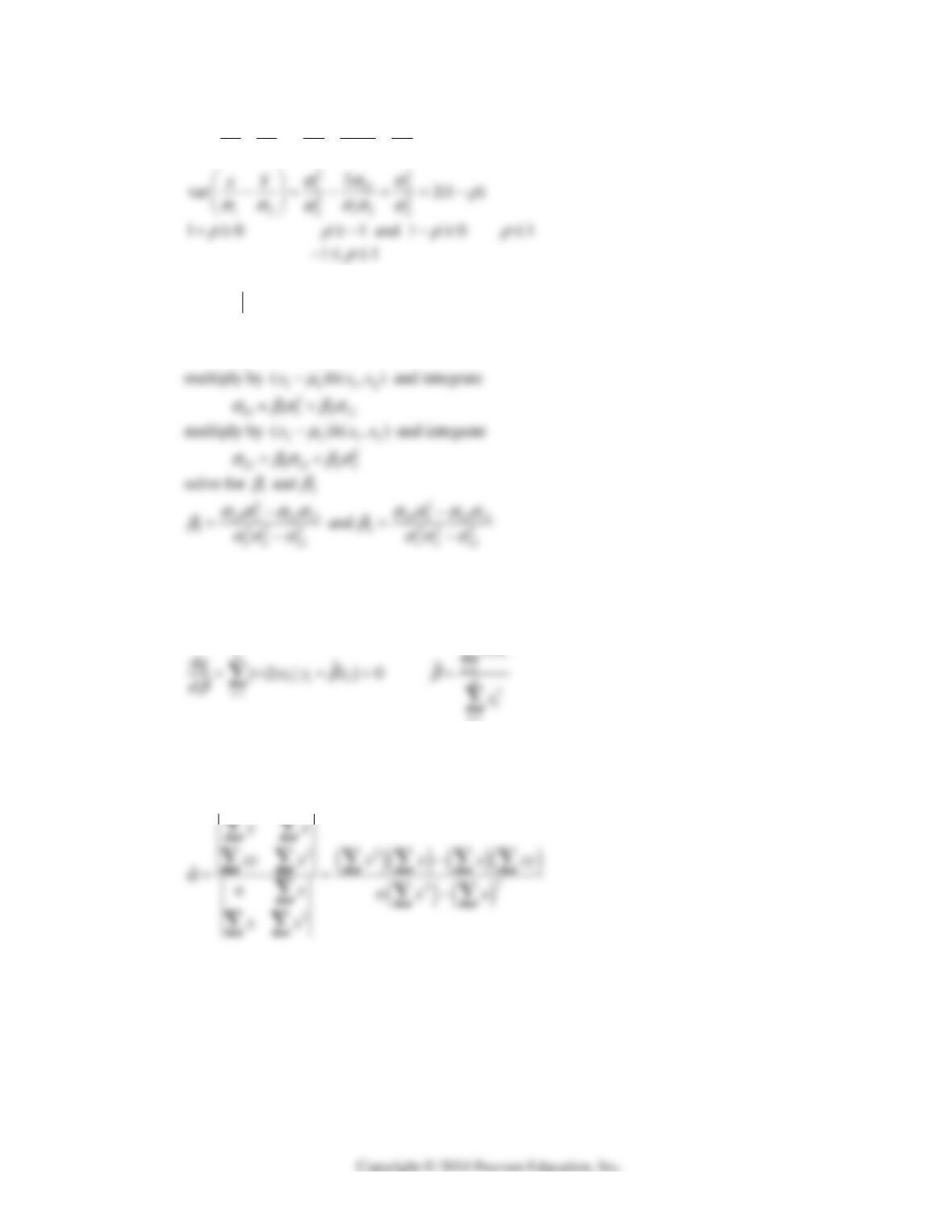
multiply by g(x) and integrate over x
22
var( ) ( ) { ( ){ ( ) [ ( )] }Yx gx dx gx EY x EYx dx
22
var( ) ( ) ( )[ ( )]
Yx EY g x EY x dx
Chapter 14 203
14.11
22
1122
2
22 122
1
2
var 2(1 )
xY
σσσ
ρ
σσ σσσ
σ
ρ
ρ
ρ
ρ
14.12
33123 111 22 2
(,) ( )( )xg x x x dx x x
αβ µ β µ
multiply by
12
(, )hx x
and integrate over
12 3
, and xx x
2
00
µ
αα
µ
µ
β
14.13
2
1
1
ˆ
[]
n
i
i
qyx
β
n
xy
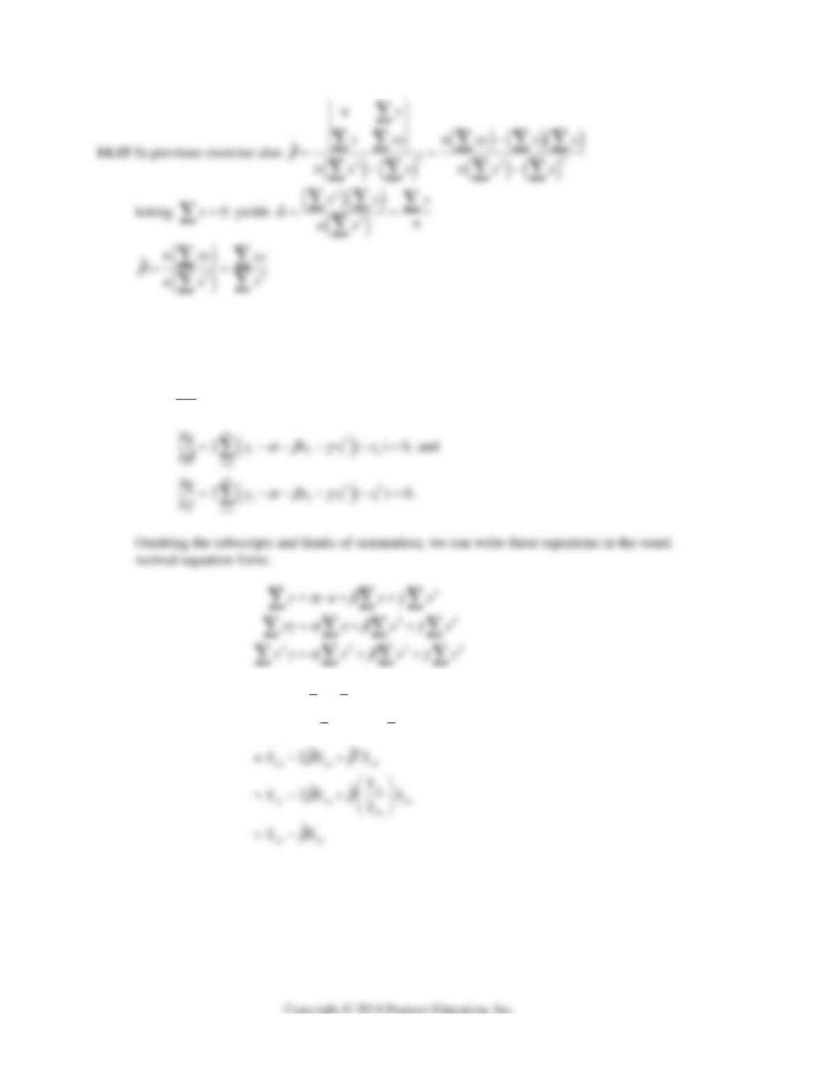
14.14
ˆ
ˆ
yn x
αβ
2
ˆ
ˆ
xy x x
αβ
204 Mathematical Statistics, 8E
14.16
22
1
2( )
n
i
i
qe y xx
αβ γ
differentiating partially with respect to
, and
αβ γ
and
setting the resulting derivatives to zero to obtain the maximum likelihood estimates, we obtain
2
1
2(1)0,
n
iii
i
qyxx
αβ γ
α
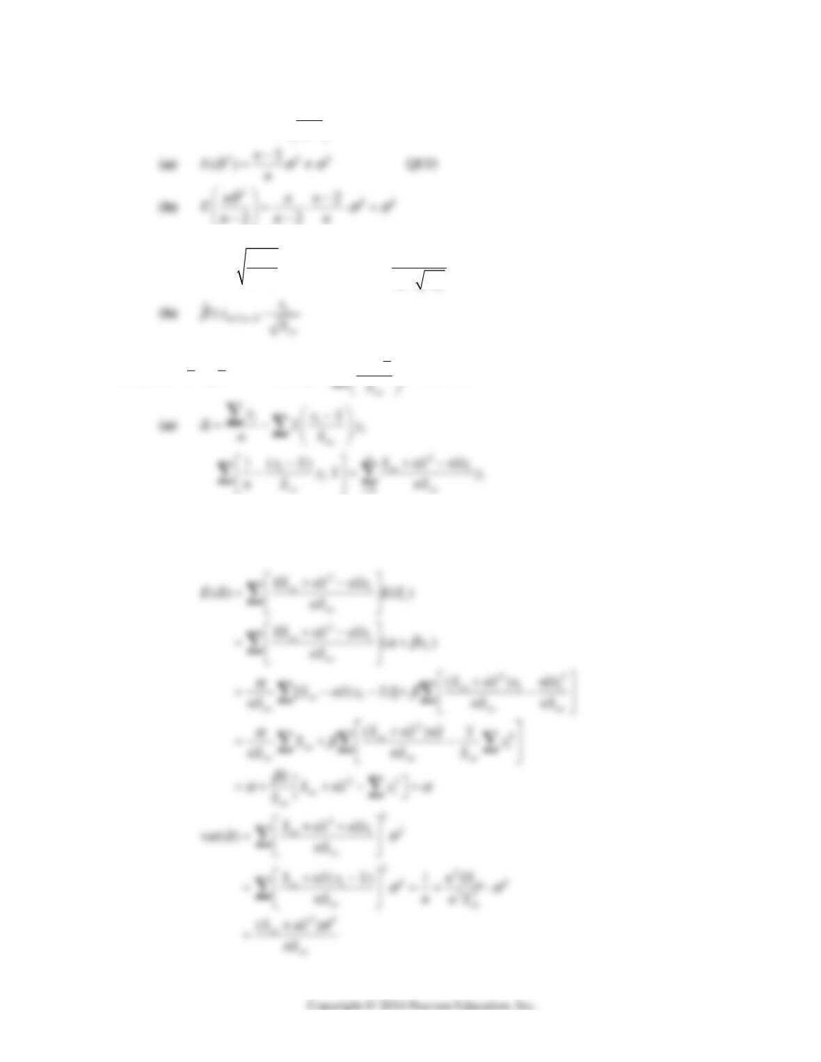
14.17
22
ˆˆˆ
ˆ
[( )] ( ]
ii
yx yyxx
αβ β β
2
ˆ
[( ) ( )]
ii
yy xx
β
Chapter 14 205
14.18 by Theorem 14.3
2
2
ˆ2
n
En
σ
σ
14.19 (a)
ˆ
ˆ
2/
e
exx
n
st
nsS
β
β
σ
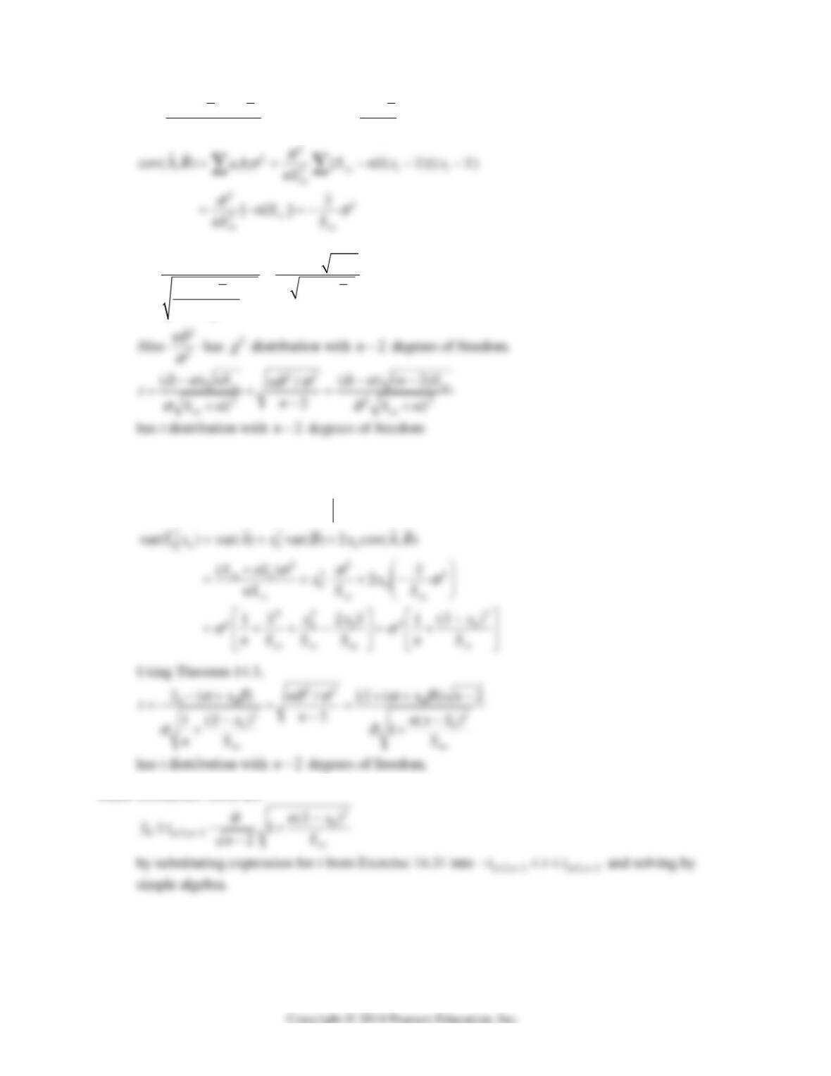
14.20 ˆ
ˆyx
αβ
with ˆ
i
xx
y
β
from text
(b) Use corollary to Theorem 4.14 and Exercise 7.58
Since
ˆ
A is linear combination of y‘s
ˆ
α
has normal distribution.
206 Mathematical Statistics, 8E
14.21
()
xx i
i
xx
Snxxx
anS
i
i
xx
xx
bS
14.22
22
ˆ
ˆ()
()
xx
xx xx
xx
nS
z
Snx Snx
nS
αα
αα
σ
σ
has standard normal distribution and is independent of Z.
14.23
00
ˆ
ˆˆ
YABx
is sum of independent normal random variables and according to Ex. 7.58 has
normal distribution
0000
ˆˆˆ
() () ( )EA xEB x EY x
αβ
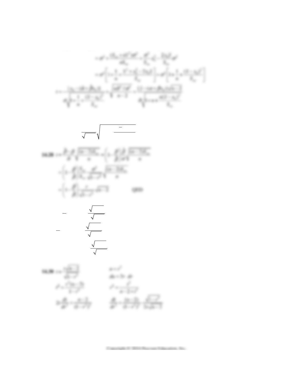
14.24 confidence limits are
Chapter 14 207
14.25
00 0 0
ˆˆ
[( )]( )( )0
EY A Bx x x
αβ αβ
22
00 0 0
ˆˆ
ˆˆ
var[ ( )] var( ) var( ) 2 cov( , )
YABx Ax B x AB
σ
14.26 Simple algebra leads to the following limits of prediction:
2
0
0/2,2
ˆ()
ˆ1
2
n
xx
nx x
yt n S
n
α
σ
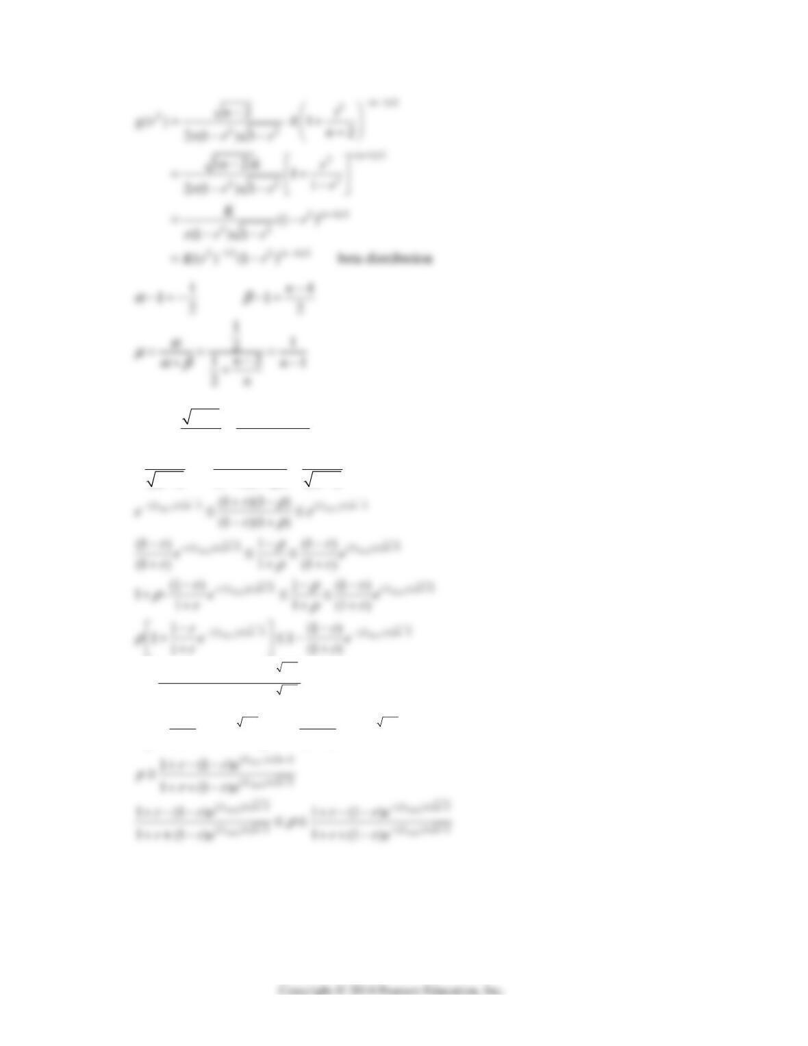
14.29
2
/2, 2
1
1ˆ2
an
r
trn
β
β
2
/2, 2
2
/2, 2
1
1
ˆ2
1
ˆ1 QED
2
an
n
r
trn
r
trn
α
β
β
ββ
208 Mathematical Statistics, 8E
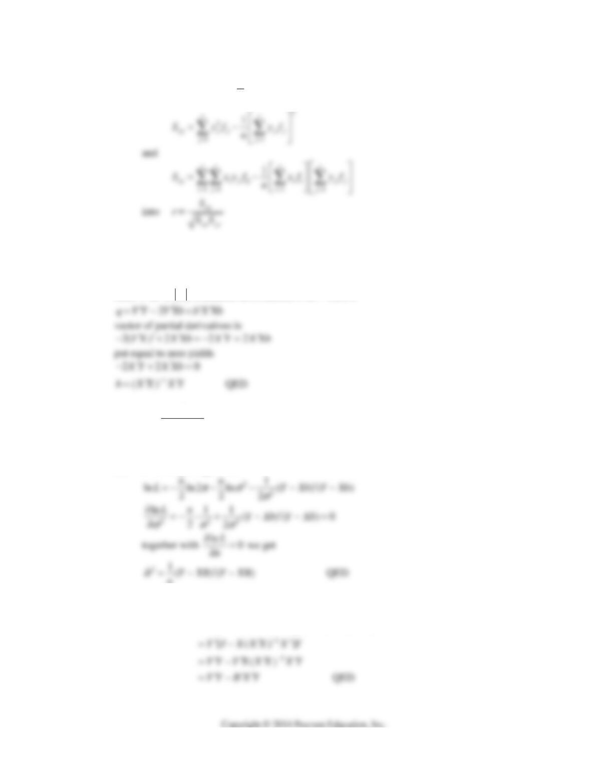
14.31
/
2/2
3(1)(1 )
ln
2(1)(1)
nr
zz
r
αα
ρ
ρ
/2 /2
2(1)(1)2
ln (1 )(1 )
33
zrz
r
nn
αα
ρ
ρ
/2
/2
/2 /2
(2 )/ 3
(2 )/ 3
(2 )/ 3 (2 )/ 3
1(1) and
1(1)
1(1)
11
1(1)
zn
zn
zn zn
rre
rre
rr
ee
rr
α
α
αα
ρ
ρ
Chapter 14 209
14.32 Substitute
2
2
11
1
rr
xx i i i i
ii
Sxf xf
n
14.33
()()
{()}{ }
() ()
qYXbYXb
YXbYXb
Y Y Y Xb Xb Y Xb Xb
since
is , a number, not a matrix, ( )YXb X YXb Xb Y
14.34
2
2(1/2)()()
2/2
1
(, ) (2 )
Yxb YXb
n
Lb e
σ
σπσ
To maximize L minimize
()()YXbYXb
as in Ex 14.33
(a)
maximum likelihood estimates = least square estimates
(b) as in simple regression
n
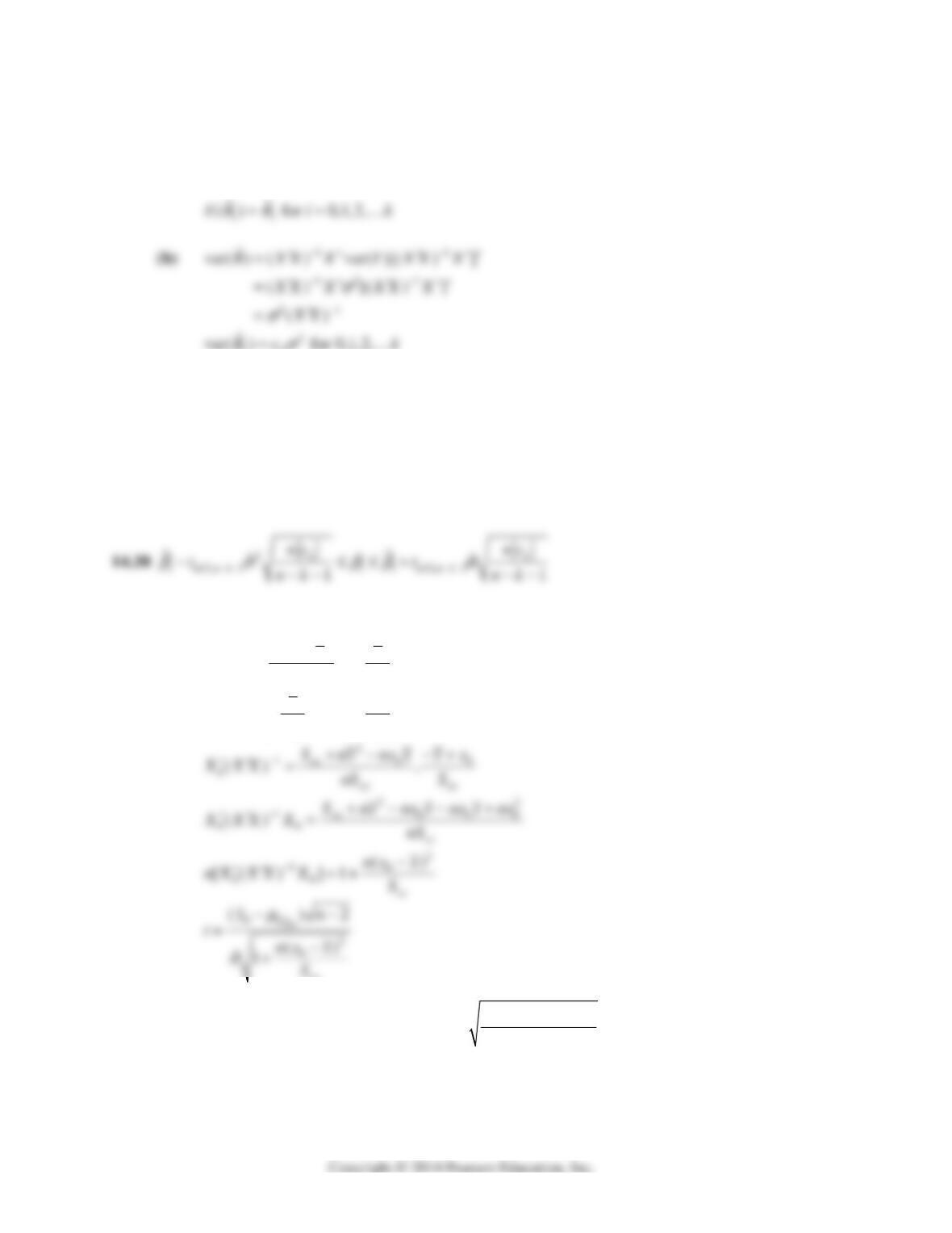
14.35
11
11
()()[(()][()]
[()][()]
YXBYXB YXXX XYYXXX XY
YI XXX X I XXX XY
210 Mathematical Statistics, 8E
14.36
1
ˆ()BXXXY
(a)
1
1
ˆ
() ( ) ()
()
E B XX XE Y
XX XXB B
1
ii
(c)
11
12 1
21
ˆ
cov( ) ( ) cov( )[( ) ]
() [() ]
()
B XXX YXXX
XX I XX X
xx
σ
σ
2
ˆˆ
cov( , ) for 0,1,
ij ij
BB c i j k
σ
14.39 (a)
00010
ˆˆ
ˆˆ
ˆ
()()BX X x y
αβ α β
2
1
() 1
xx
xx xx
xx xx
Snx x
nS S
XX x
SS
xx
(b) confidence limits are
1
00
0/2,1
[( )
ˆ1
nk
nX XX X
BX t nk
α
σ
Chapter 14 211
14.40 (a) From 14.39
00
ˆ
ˆ
BX X
αβ
(b) confidence limits are
1
00
0/2,1
[1 ( ) ]
ˆ1
nk
nXXXX
BX t nk
α
σ
14.41 (a)
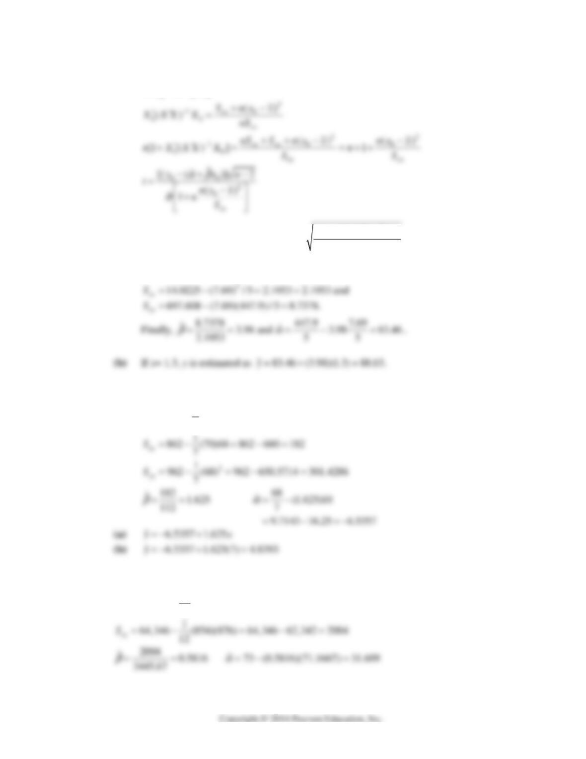
2
5, 7.69, 14.0225, 447.9, 697.608nx x y xy
Thus,
14.42 (a)
22
7, 70, 812, 68, 952, 862nx x y y xy
2
1
812 (70) 812 700 112
7
xx
S
14.43
22
12, 854, 64.222, 876, 65,850, 64,346nx x y y xy
2
1
64,222 (854) 64,222 60,776.333 3445.67
12
xx
S
212 Mathematical Statistics, 8E
(a)
ˆ31.609 0.5816
yx
(b)
ˆ31.609 0.5816(84) 80.45
y
14.44
22
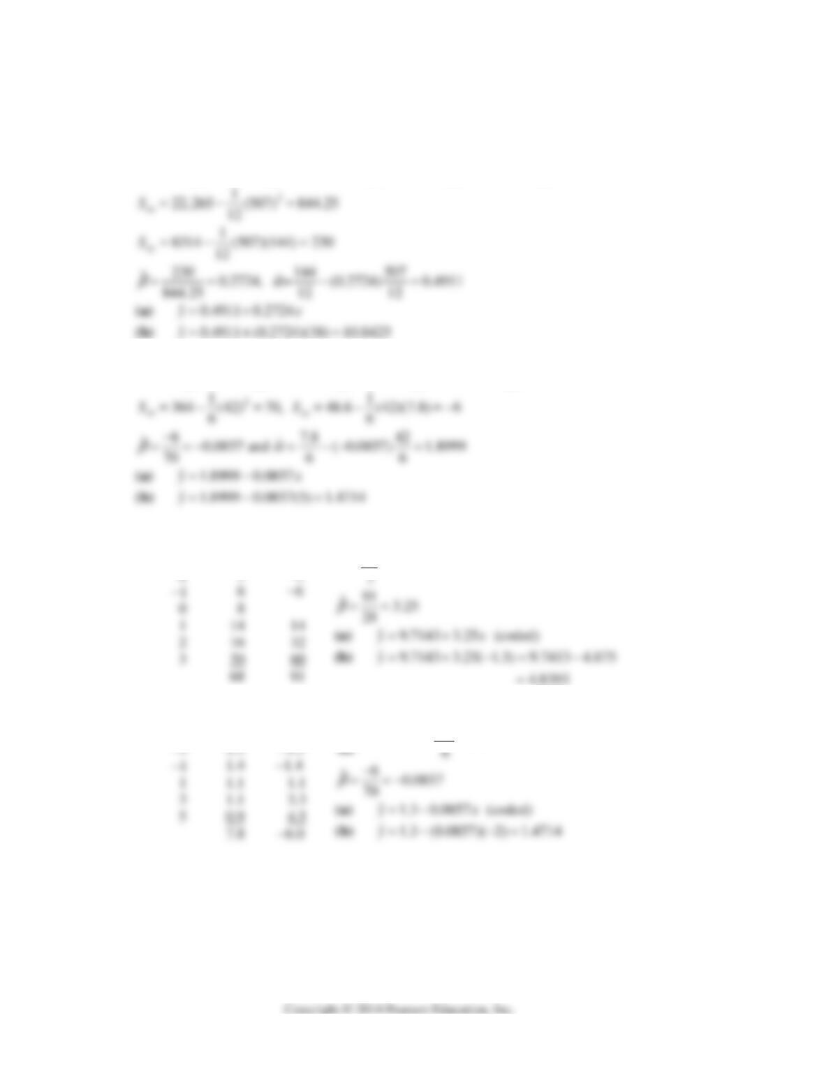
12, 507, 22,265, 144, 1802, 6314nx x y y xy
14.45
22
6, 42, 364, 7.8, 10.68, 48.6nx x y y xy
14.46
x
y
xy
3
1
3
2
3
6
68
ˆ9.7143
α
14.47
x
y
xy
5
1.8
9.0
2
7.8
ˆ
70, 1.3
x
α