Chapter 13
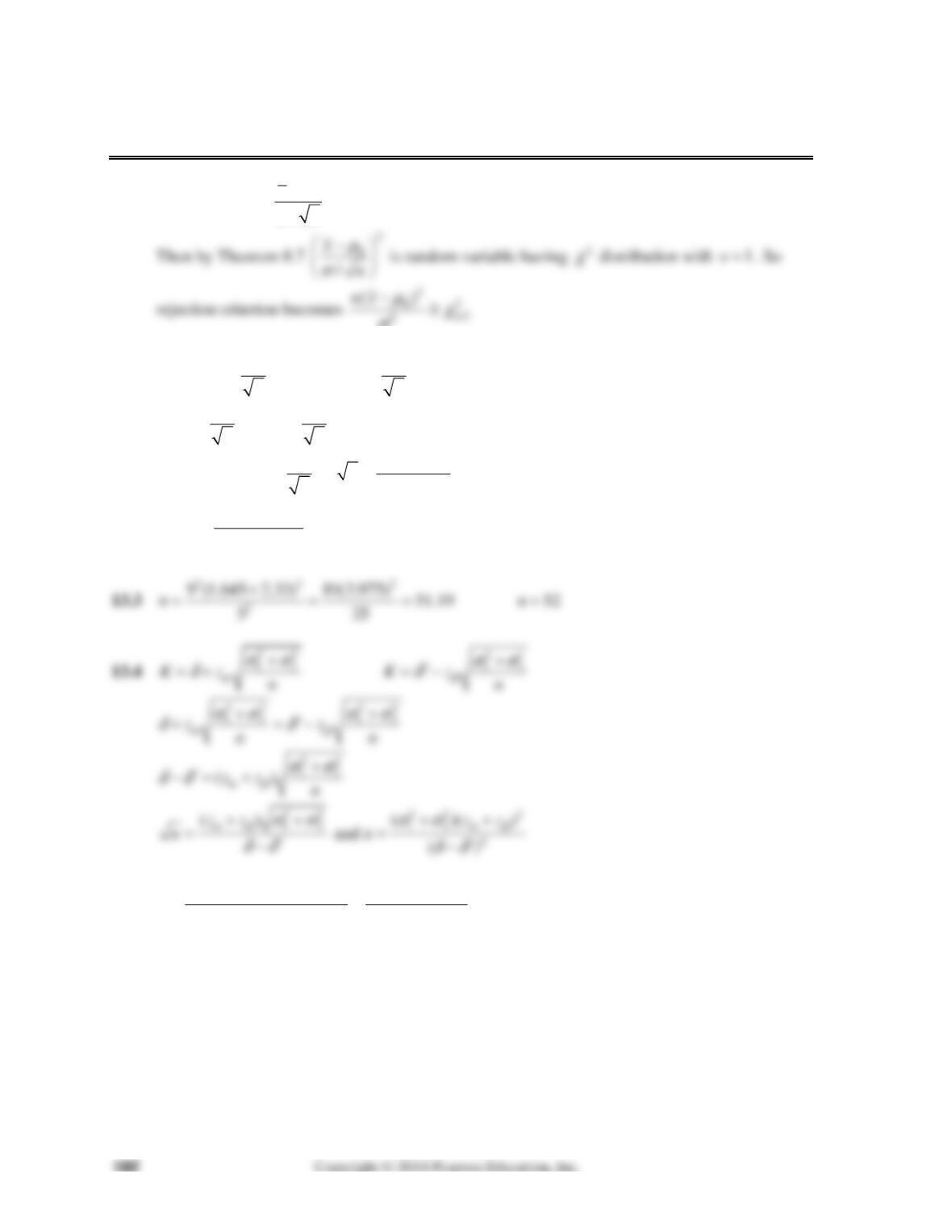
13.1 Test statistic
0
/
x
zn
μ
σ
χ
σ
13.2
01
and Kz Kz
nn
αβ
σσ
μμ
01
zz
nn
αβ
σσ
μμ
10
10
()
() zz
zz n
n
αβ
αβ
σ
σ
μμ
μ
μ
and
22
2
10
()
()
zz
n
αβ
σ
μμ
13.5
2
2
(81 169)(2.33 2.33) (250(21.7156) 150.80 151
36
6
n
Chapter 13 183
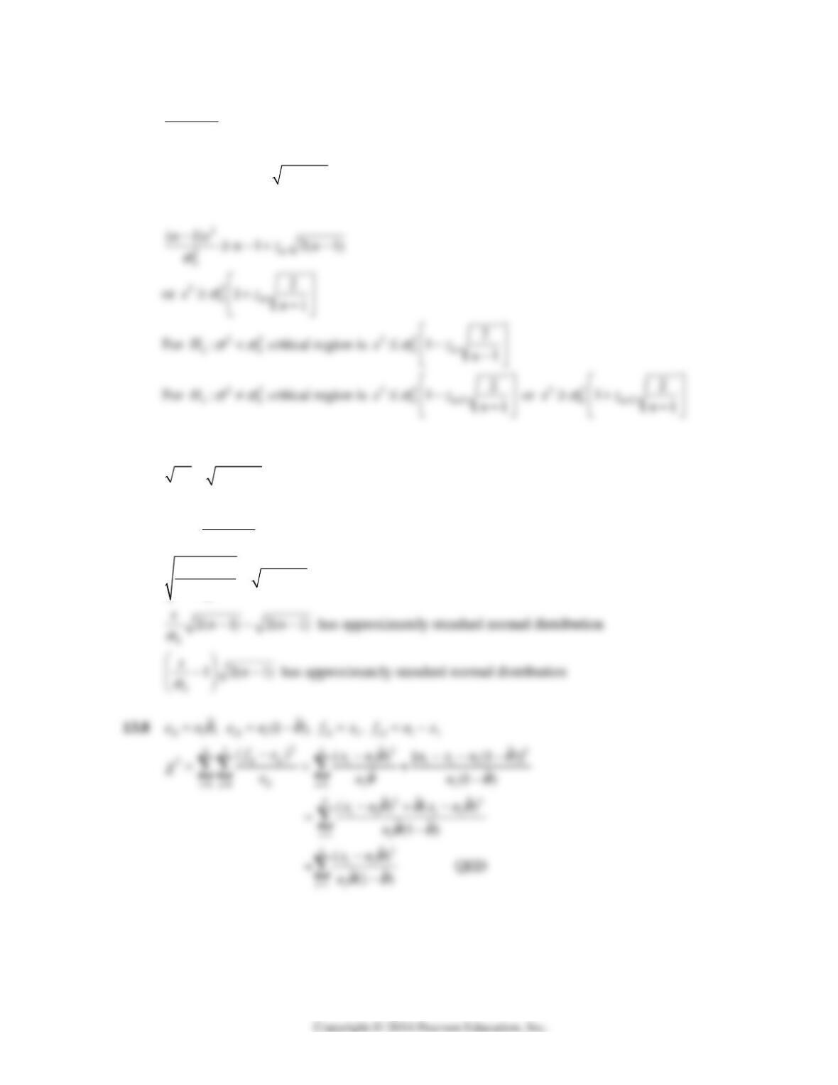
13.6
2
2
0
(1)ns
σ
has chi square distribution with (1)n degrees of freedom, so that according to
corollary 2 to Theorem 6.3
1 and 2( 1)nn
μσ
Using normal approximation, critical region is
13.7 If x has
2
χ
distribution with
1n
degrees of freedom, then according to Example 8.42
22(1)xn
standard normal distribution.
Since
2
2
0
(1)ns
σ
has chi square distribution with
1n
degrees of freedom.
2
2
0
2( 1) 2( 1)
ns n
σ
has approximately standard normal distribution
184 Mathematical Statistics, 8E
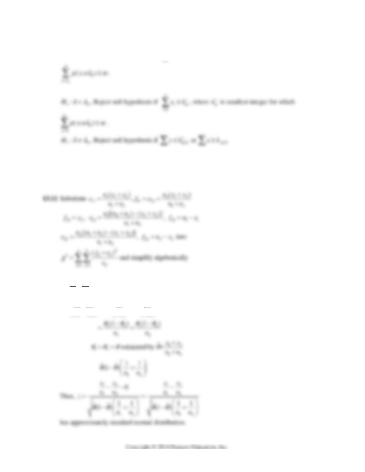
13.9
10
:H
λλ
, Reject null hypothesis if
n
i
xk
α
, where
k
α
is smallest integer for which
13.10 From Table II with
5(3.6) 18
λ
0.025
25k
(Probability
28 0.0173, 27 0.0282)Xx
0.025
9k
(Probability
9 0.0153, 10 0.0303)Xx
13.12
12
12
12
0
xx
Enn
θθ
12 1 2
var var var
xx x x
nn n n
Chapter 13 185
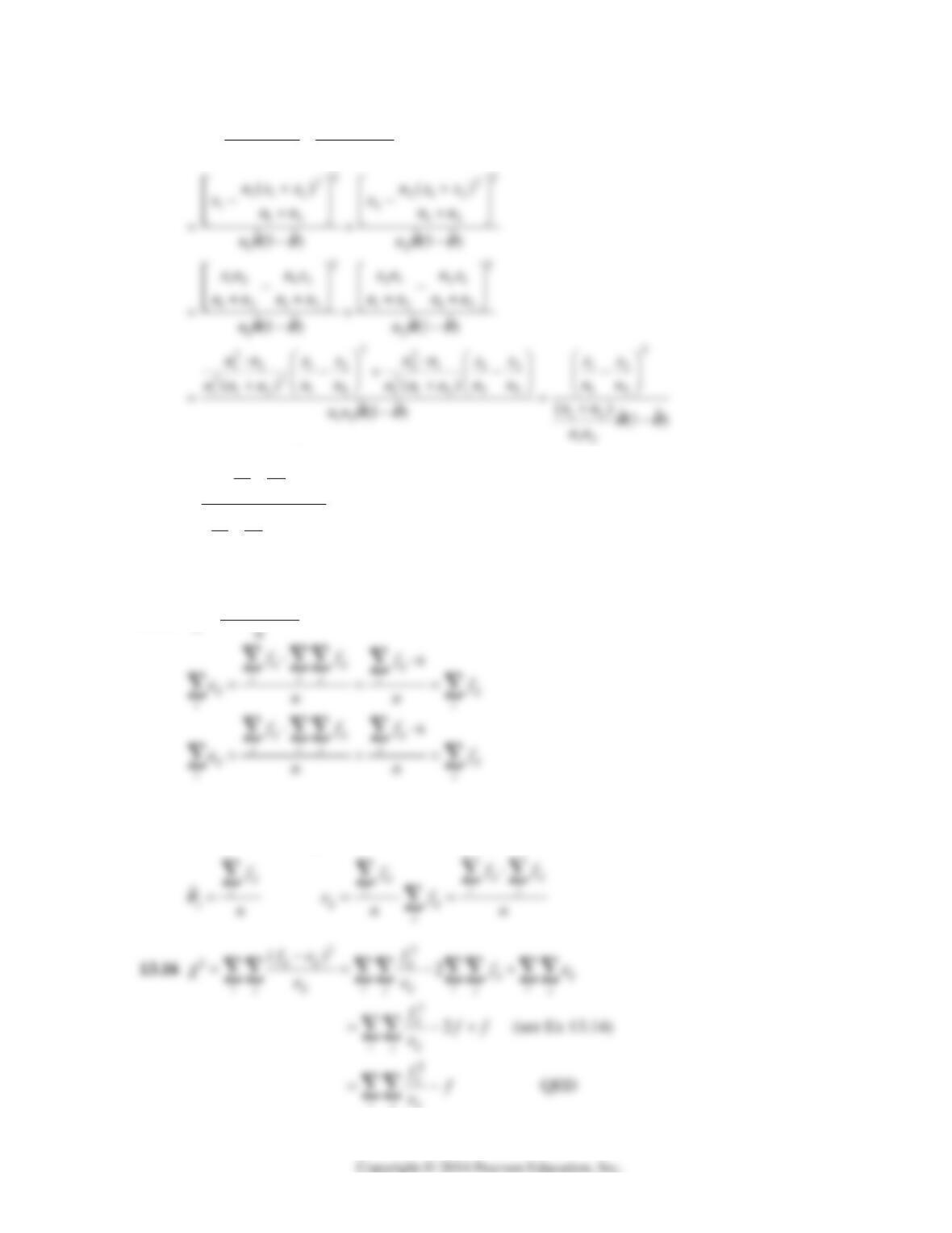
13.13
22
211 2 2
12
ˆˆ
()( )
ˆˆ ˆˆ
(1 ) (1 )
xn xn
nn
θθ
χθθ θθ
2
12
12 2
12
QED
11
ˆˆ
(1 )
xx
nn Z
nn
θθ
13.14
ij ij
ij
ij
ff
en
13.15 Under
12
: for 1,2, .
oj j nj
He j
θθ
j
θ
ij
ij
186 Mathematical Statistics, 8E
13.17
222222
2
232 260 197 168 240 203 1300
212 265 212 188 235 188
253.887 255.094 183.061 150.128 245.106 219.197 1300
6.473 (differs due to rounding)
χ
13.19 (a) not necessarily; (b) yes
13.20 (a) No, since 0.0316 > 0.01
13.21 Normal curve area corresponding to
2.84z
is 0.4977
p-value is
2(0.5000 0.4977) 0.0046
13.23 p-value is
1 0.3502 0.3249
2
. As is exceeds 0.05, null hypothesis cannot be rejected.
Chapter 13 187
μ
13.26 2.
0
/
x
zn
μ
σ
3.
87.5 84.3 2.73
8.6 / 45
z
, p-value =
0.5000 0.4968 0.0032
4. Since
0.0032 0.01
, null hypothesis must be rejected.
μ
13.28 2.
0
/
x
zn
μ
σ
3.
30.8 30 3.02
1.5 / 32
z
, p-value =
2(0.5 0.4987) 0.0026
4. Since 0.0026 is less than 0.005, null hypothesis must be rejected.
μ
13.30
5, 14.4, 0.158nx s
1.
01
:14, :14, 0.05HH
μ
μα
2. Reject null hypothesis if
2.776 or 2.776tt
3.
14.4 14 5.66
0.158 / 5
t
4. Since 5.66 exceeds 2.776, null hypothesis must be rejected.
μ
188 Mathematical Statistics, 8E
13.32
5.66, d.f. 4t
p-value =
1 0.9952 0.0048
Since
0.0048 0.05
, null hypothesis must be rejected.
13.34 (a)
00
(reject on exactly one factor is true for all 48 factors)PH H
147
48 (0.01) (0.99) 0.30
1
(b)
00
(reject on more than one factor is true for all 48 factors)PH H 1 0.30 0.70
.
13.35
12
22
( ) 0.20 1.96 or 1.96
(0.12) (0.14)
50 40
xx
12
( ) 0.20 1.96 or 1.96
0.0279
xx
12
0.20 0.0547 0.145
xx
or
12
0.20 0.0547 0.255
xx
Chapter 13 189
13.36 1.
01 2 11 2
:0, :0, 0.05
HH
μ
μμμα
13.37
2.60, value 2(0.5 0.4953) 0.0094
zp
Since
0.0094 0.05
, null hypothesis must be rejected.
13.38 1.
01 2 11 2
: 0.05, : 0.05, 0.05
HH
μ
μμμα
13.39
1.22, value 0.5 0.3888 0.1112
zp
Since
0.1112 0.05
, null hypothesis cannot be rejected.
13.40 1.
01 2 11 2
:0, :0, 0.01
HH
μ
μμμα
2. Reject null hypothesis if
0.005 0.005
3.169 or 3.169
tt tt
13.41 2.67, d.f. 6, 0.05
t
α
p-value = 1(1 0.9630) 0.0185
2
13.42
11 2 2
144, 19.06, 149, 14.21
xs xs
1.
01 2 11 2
:, :, 0.01
HH
μ
μμμα
190 Mathematical Statistics, 8E
13.43 0.52, d.f. 10
t
p-value = 1 0.3856 0.61
Since
0.61 0.01,
null hypothesis cannot be rejected.
13.44 13, 7, 1
, 5, 3, 2, 1
, 0, 6, 1, 4, 3, 2, 6, 12, 4
4.125, 4.064, 16
xsn
1.
: 0, : 0, 0.05
HH
μ
μα
13.45 9, 13, 2, 5, 2
, 6, 6, 5, 2, 6
10, 5.2, 4.08
nx s
1.
01
: 0, : 0, 0.05
HH
μ
μα
13.46 4.03, d.f. 9
t
p-value 1(1 0.997) 0.0015
2
13.47 1.
01
: 0.0100, : 0.0100, 0.05
HH
σσα
2. Reject null hypothesis if
22
2.733
χχ
4. Since
5.92 2.733
, null hypothesis cannot be rejected.
13.48 238, 24
sn
1.
01
: 250, : 250, 0.01
HH
σσα
13.49 2.53, 30, =0.05
sn
α
1.
01
: 2.85, : 2.85, 0.05
HH
σσα
Chapter 13 191
13.50 1.
0010
:, :, 0.05
HH
σσ σσα
2. Reject null hypothesis if
0.05
1.645
zz
13.51 50, 0.49
ns
1.
01
: 0.41, : 0.41, 0.05
HH
σσα
Since
0.0268 0.05
, null hypothesis must be rejected.
13.53
11 2 2
4, 31, 4, 26, 0.05
ns ns
α
1.
01 2 11 2
: 0, : 0, 0.05
HH
σσ σσ α
13.54 1.
01 2 11 2
: 0, : 0, 0.10
HH
σσ σσ α
13.55
1212
19.06, 14.21, 6
ssnn
1.
01 2 11 2
: 0, : 0, 0.02
HH
σσ σσ α
192 Mathematical Statistics, 8E
13.56 20, 0.5 against 0.50, 0.05
n
θθα
( 5) 0.0207
px
Critical region is 5 or 15
xx
13.57 1.
01
:0.40, :0.40, 0.05
HH
θθα
2. Observed number of successes in n = 18 trials
13.58 ( 12) 0.0203
pX
Critical region is 12
x
13.59 1.
01
:0.30, :0.30, 0.05
HH
θθα
2. Observed number of successes in n = 19 trials
13.60 ( 2) 0.0462
px
Critical region is 2
x
( 3) 0.1331
px
0.0462
α
13.61 1.
:0.40, :0.40, 0.01
HH
θθα
13.62 ( 0) 0.0008, ( 11) 0.0039
Px Px
, Critical region is x = 0, or 11
x
( 1) 0.0081, ( 10) 0.0175
Px Px
, 0.008 0.0039 0.0047
α
13.63
01
:0.35; :0.35.
HH
θθ
Using the normal approximation
13.64 1.
01
:0.20, :0.20, 0.01
HH
θθα
2. Number of successes in n = 12 trials
Chapter 13 193
13.65 1.
01
:0.60, :0.60, 0.05
HH
θθα
13.66 1.
01
:0.30, :0.30, 0.05
HH
θθα
13.67 1.
01
:0.90, :0.90, 0.05
HH
θθα
13.68 1.
01 2 11 2
:, :, 0.01
HH
θθ θθα
2. Reject null hypothesis if
22
0.01,1
6.635
χχ
11
166 250 83,
500
e
others by subtraction
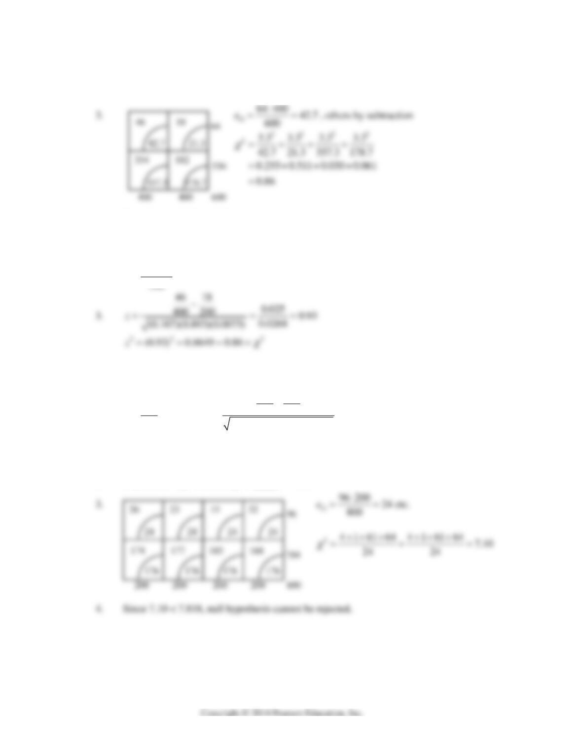
13.69 1.
01 2 11 2
:, :, 0.01
HH
θθ θθα
2. Reject null hypothesis if
0.005 0.005
or
zz zz
194 Mathematical Statistics, 8E
13.70 1.
01 2 11 2
:, :, 0.05
HH
θθ θθα
2. Reject null hypothesis if
22
0.05,1
3.841
χχ
4. Since 0.86 < 3.841, null hypothesis cannot be rejected.
13.71 1.
01 2 11 2
:, :, 0.05
HH
θθ θθα
2. Reject null hypothesis if 1.96 or 1.96
zz
74 92
ˆ0.332
θ
13.72
01 2 11 2
:, :, 0.05
HH
θθ θθα
2. Reject null hypothesis if 1.645
z
3. 169
ˆ0.338
500
θ
82 87
200 300 2.78
(0.338)(0.662)(0.00833)
z
4. Since 2.78 > 1.645, null hypothesis must be rejected.
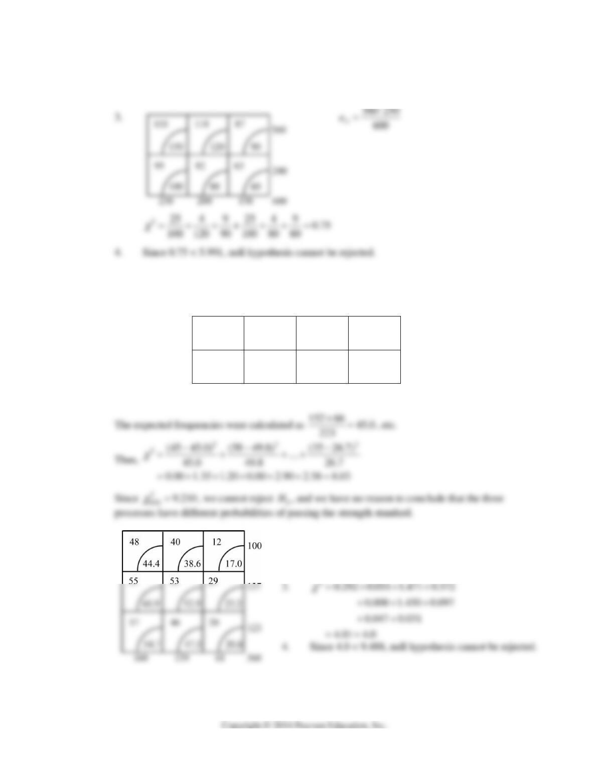
13.73
01 2 3 4 1
:, :
HH
θθθθ
not all equal, 0.05
α
2. Reject null hypothesis if
22
0.05,3
7.815
χχ
Chapter 13 195
13.74
01 2 3 1
:, :
HH
θθθ
not all equal, 0.05
α
2. Reject null hypothesis if
22
0.05,2
5.991
χχ
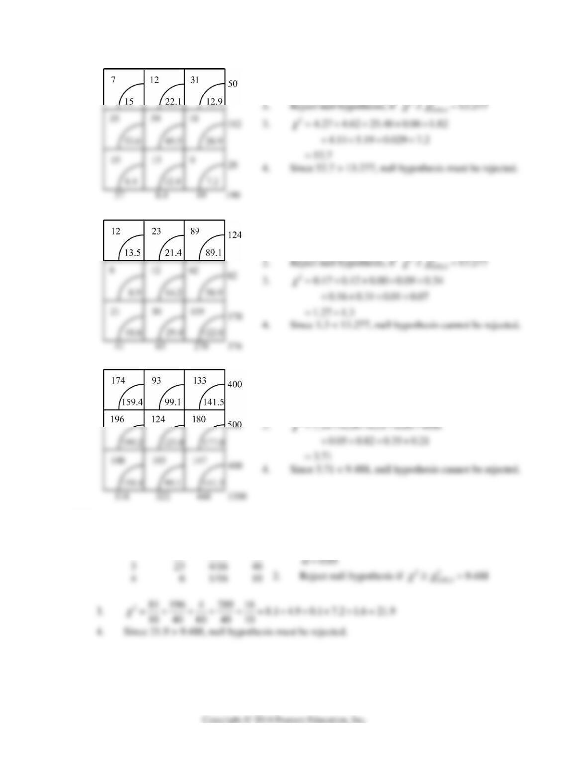
13.75 In the following contingency table, the expected frequency is given below the observed
frequency in each cell.
TOTALS
45
45.0
58
49.8
49
57.3 152
21
21.0
15
23.2
35
26.7 71
TOTALS 66 73 84 223
13.76 1.
0
:
H
independent,
1
:
H
not independent,
0.05
α
2. Reject null hypothesis, if
22
0.05,4
9.488
χχ
196 Mathematical Statistics, 8E
13.77 1.
0
:
H
independent,
1
:
H
not independent,
0.01
α
22
13.78 1.
0
:
H
Venders ship equal quantities
1
:
H
Venders do not ship equal quantities;
0.01
α
13.79 1.
0
:
H
percentages same for three cities
1
:
H
percentages not same for three cities
0.05
α
2. Reject null hypothesis, if
22
0.05,4
9.488
χχ
2
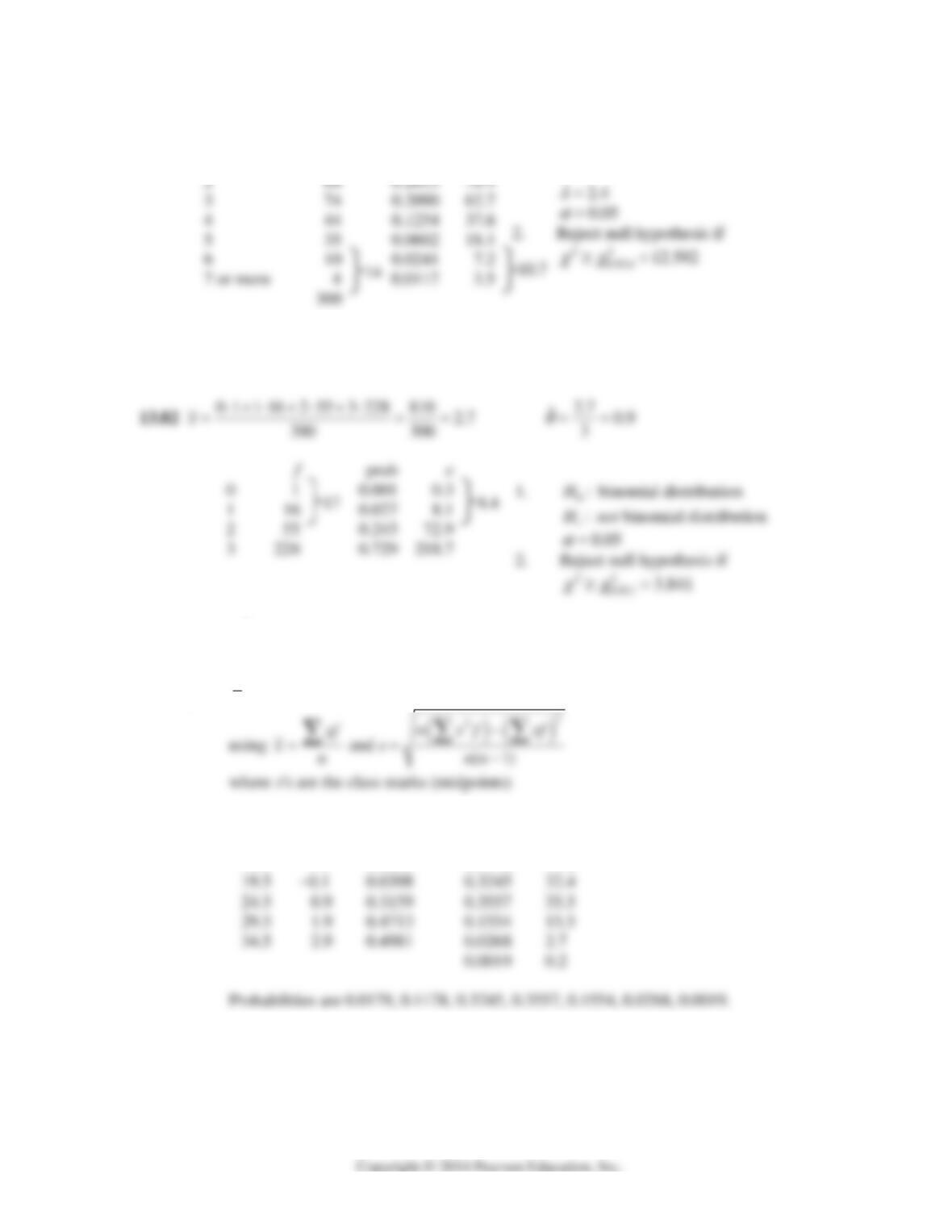
13.80 f prob e
0 19 1/16 10
1 54 4/16 40
2 58 10/16 60
1.
0
:
H
coins are balanced
1
:
H
coins are not balanced
Chapter 13 197
13.81 f prob e
0 19 0.0907 27.2
1 48 0.2177 65.3
1.
0
:
H
Poisson distribution with
2.4
λ
1
:
H
not Poisson distribution with
3.
2
2.47 4.58 1.96 2.04 1.09 15.78 1.02 28.9
χ
4. Since 28.9 > 12.592, null hypothesis must be rejected.
3.
2
8.80 4.40 0.40 13.6
χ
4. Since 13.6 > 3.841, null hypothesis must be rejected.
13.83 (a)
20 and 5.025 5
xs
(b) z e
9.5
2.1
0.4821 0.0179 1.8
14.5
1.1
0.3643 0.1178 11.8
198 Mathematical Statistics, 8E
(c) Expected frequencies are 1.8, 11.8, 32.4, 35.6, 15.5, 2.7, 0.2
1.
0
:
H
normally distributed random variables
:
A
H
not normally distributed random variables,
0.05
α
13.84
01
: 300; : 300.
HH
μ
μ
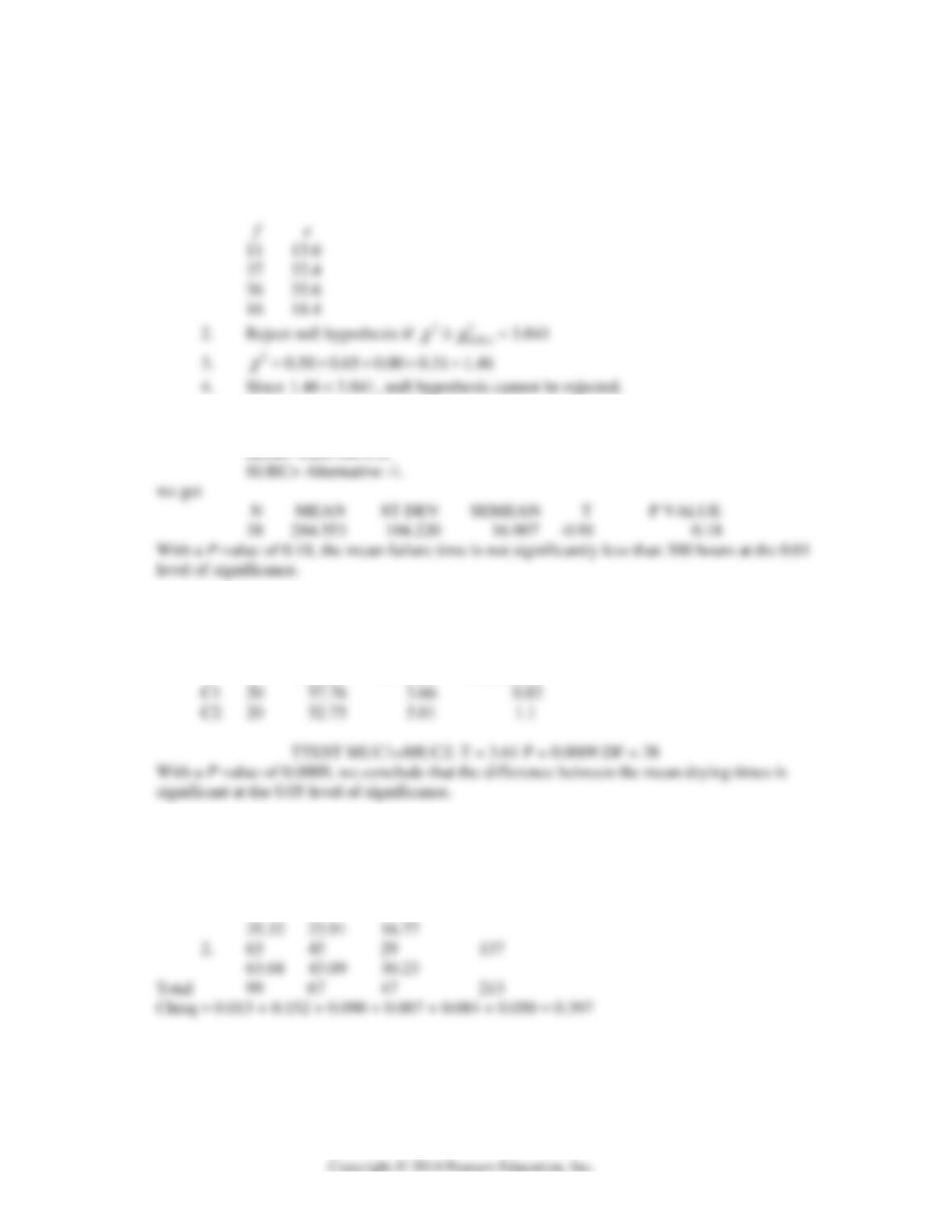
Using MINITAB:
13.85
01 2 11 2
:; :
HH
μ
μμμ
Using MINITAB:
MTB> TwosampleT for C1 vs C2
we get
N MEAN ST DEV SEMEAN
13.86 Using MINITAB, we enter the three columns in this table into C1, C2, and C3, respectively.
MTB> Chisquare C1 C2 C3
Expected counts are printed below observed counts.
C1 C2 C3 Total
1 36 22 18 76
From Table V with df = 2,
2
0.05,2
5.991
χ
, and we cannot reject the null hypothesis that the
three materials have the same probability of leaking at the 0.05 level of significance.