11.4.14.
(a)u(x) = 8
<
:−1.25(x+ 1)3+ 4.25(x+ 1) −2,−1≤x≤0,
1.25x3−3.75x2+.5x−1,0≤x≤1.
-1 -0.5 0.5 1
-2
-1.5
-1
-0.5
0.5
1
2
1.5 2 2.5 3 3.5 4
(d)u(x) =
8
>
>
>
>
>
>
>
<
>
>
>
>
>
>
>
:
1.53571(x+ 2)3−4.53517(x+ 2) + 5,−2≤x≤ −1,
−3.67857(x+ 1)3+ 4.60714(x+ 1)2+.07143(x+ 1) + 2,−1≤x≤0,
4.17857x3−6.42857x2−1.75x+ 3,0≤x≤1,
−2.03571(x−1)3+ 6.10714(x−1)2−2.07143(x−1) −1,1≤x≤2.
2
3
4
5
333
The particular solutions are:
(a)u(x) = 8
<
:−5.25(x+ 1)3+ 8.25(x+ 1)2−2,−1≤x≤0,
4.75x3−7.5x2+.75x+ 1,0≤x≤1.
-1 -0.5 0.5 1
-2
-1.5
-1
-0.5
0.5
1
2
(d)u(x) =
8
>
>
>
>
>
>
>
<
>
>
>
>
>
>
>
:
4.92857(x+ 2)3−7.92857(x+ 2)2+ 5,−2≤x≤ −1,
−4.78571(x+ 1)3+ 6.85714(x+ 1)2−1.07143(x+ 1) + 2,−1≤x≤0,
5.21429x3−7.5x2−1.71429x+ 3,0≤x≤1,
−5.07143(x−1)3+ 8.14286(x−1)2−1.07143(x−1) −1,1≤x≤2.
-2 -1 1 2
-1
1
2
3
4
5
11.4.16.
334
0.5 1 1.5 2 2.5 3
(c)u(x) =
8
>
>
>
>
>
>
>
<
>
>
>
>
>
5
4x3−9
4x2+ 1,0≤x≤1,
−3
4(x−1)3+3
2(x−1)2−3
4(x−1),1≤x≤2,
3
4(x−2)3−3
4(x−2)2,2≤x≤3,
0.2
0.4
0.6
0.8
1
♠11.4.17.
(a) If we measure xin radians,
u(x) = 8
>
>
>
>
>
<
>
>
.9959x−.1495x3,0≤x≤1,
.5 + .8730“x−1
6π”−.2348“x−1
6π”2−.297“x−1
6π”3,1
6π≤x≤1
4π,
♣11.4.18.
(a)
u(x) = 8
>
>
>
>
>
<
>
>
>
>
>
:
2.2718x−4.3490x3,0≤x≤1,
.5 + 1.4564“x−1
4”−3.2618“x−1
4”2+ 3.7164“x−1
4”3,1
4≤x≤9
16 ,
.75 + .5066“x−9
16 ”+.2224“x−9
16 ”2−.1694“x−9
16 ”3,9
16 ≤x≤1.
335
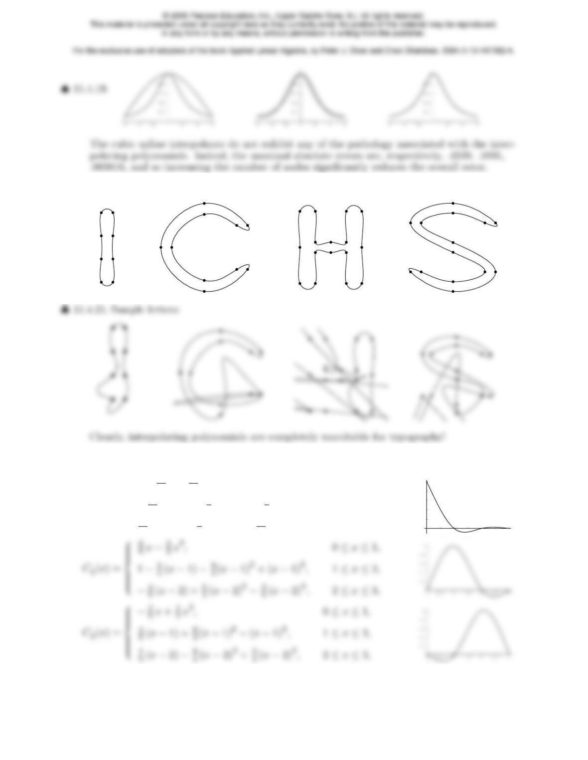
♣11.4.20. Sample letters:
♥11.4.22.
(a)
C0(x) = 8
>
>
>
>
>
<
>
>
>
>
>
:
1−19
15 x+4
15 x3,0≤x≤1,
−7
15 (x−1) + 4
5(x−1)2−1
3(x−1)3,1≤x≤2,
2
15 (x−2) −1
5(x−2)2+1
15 (x−2)3,2≤x≤3,
0.5 1 1.5 2 2.5 3
0.2
0.4
0.6
0.8
1
336
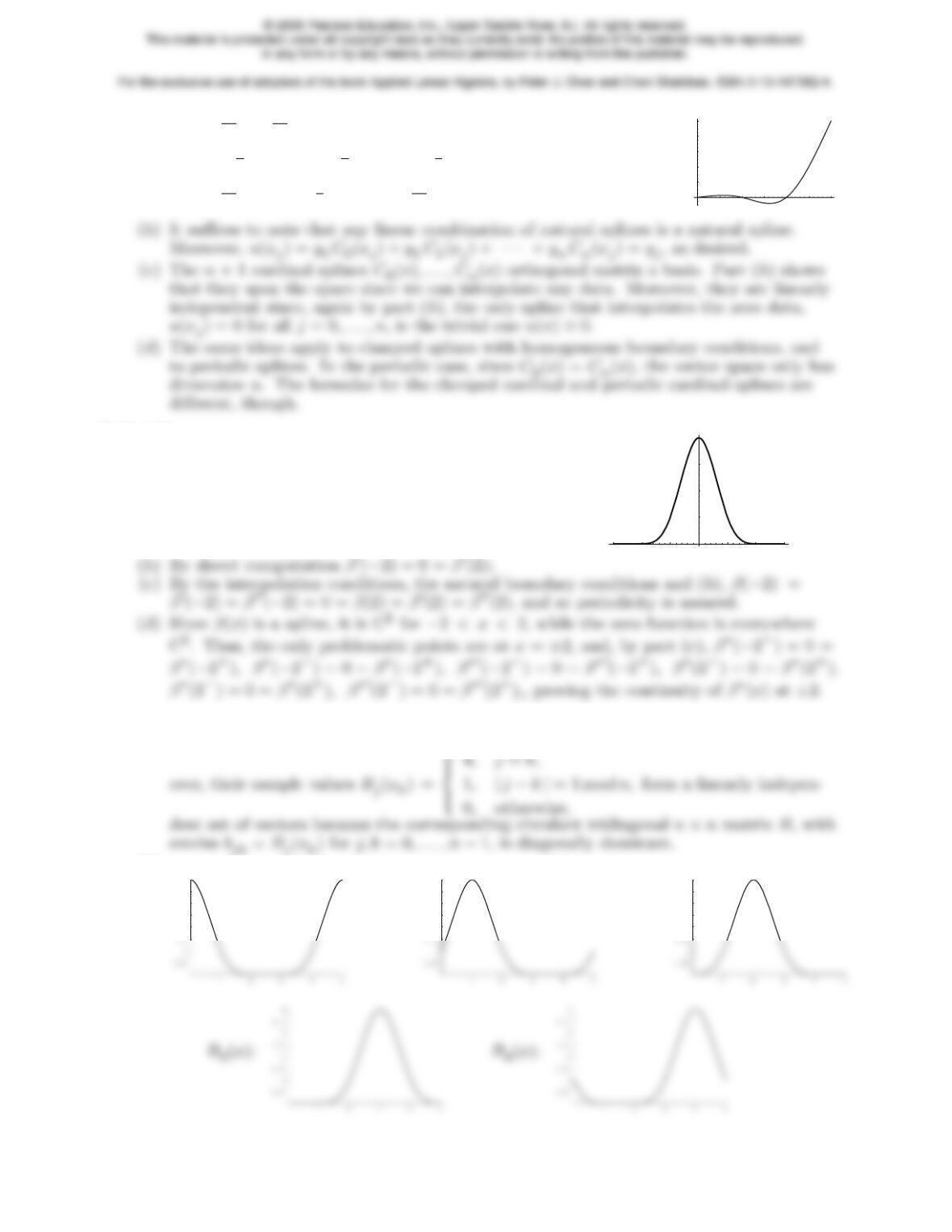
C3(x) = 8
>
>
>
>
>
<
>
>
>
>
>
:
1
15 x−1
15 x3,0≤x≤1,
−1
215(x−1) −1
5(x−1)2+1
3(x−1)3,1≤x≤2,
7
15 (x−2) + 4
5(x−2)2−4
15 (x−2)3,2≤x≤3.
0.5 1 1.5 2 2.5 3
0.2
0.4
0.6
0.8
1
♥11.4.23.
(a)β(x) =
8
>
>
>
>
>
>
<
>
>
>
>
>
>
:
(x+ 2)3,−2≤x≤ −1,
4−6x2+ 3x3,−1≤x≤0,
4−6x2−3x3,0≤x≤1,
(2 −x)3,1≤x≤2.
-3 -2 -1 1 2 3
1
2
3
4
♥11.4.24.
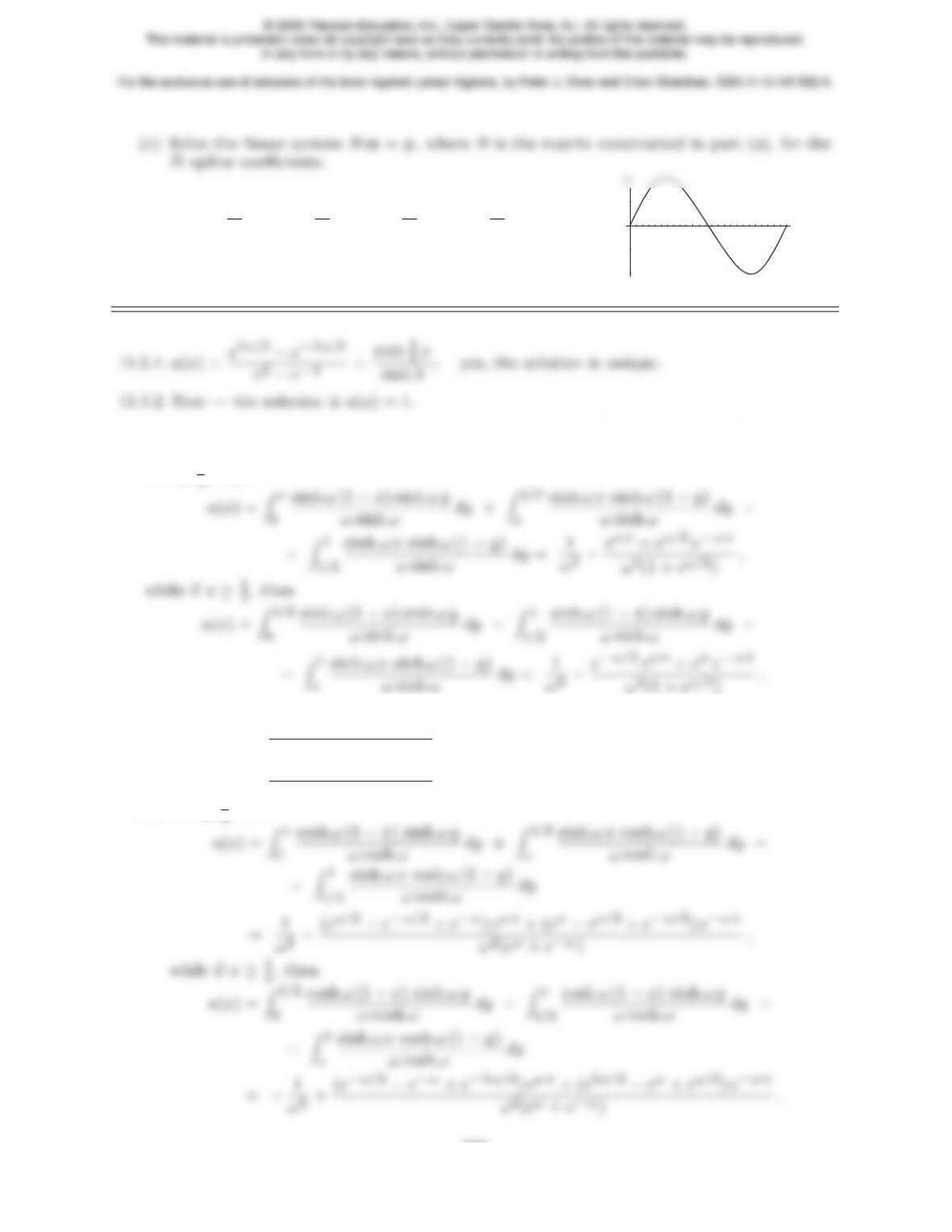
(a) According to Exercise 11.4.23, the functions Bj(x) are all periodic cubic splines. More-
(b)
B0(x):
2
2.5
3
3.5
4
B1(x):
2
2.5
3
3.5
4
B2(x):
2
2.5
3
3.5
4
337
(d)u(x) = 5
11 B1(x) + 2
11 B2(x)−2
11 B3(x)−5
11 B4(x).
12 3 4 5
-2
-1
1
11.5.3. The Green’s function superposition formula is u(x) = Z1/2
0G(x, y)dx −Z1
1/2G(x, y)dx.
If x≤1
11.5.4.
(a)G(x, y) = 8
>
>
>
<
>
>
>
:
sinh ω x cosh ω(1 −y)
ωcosh ω, x < y,
cosh ω(1 −x) sinh ω y
ωcosh ω, x > y.
(b) If x≤1
338
11.5.5.
G(x, y) = 8
>
>
>
<
>
>
>
:
cosh ω x cosh ω(1 −y)
ωsinh ω, x < y,
cosh ω(1 −x) cosh ω y
2ω,
while if x≥1
2, then
u(x) = Z1/2
0
cosh ω(1 −x) cosh ω y
ωsinh ωdy −Zx
1/2
cosh ω(1 −x) cosh ω y
ωsinh ωdy −
−Z1
x
cosh ω x cosh ω(1 −y)
ωsinh ωdy =−1
ω2+cosh ω(1 −x)
ω2cosh 1
2ω.
This Neumann boundary value problem has a unique solution since ker K= ker L=
{0}. Therefore, the Neumann boundary value problem is positive definite, and hence has
a Green’s function.
♦11.5.6. Since L[u] = “u′, u ”T, clearly ker L={0}, irrespective of any boundary conditions.
♥11.5.7.
(a) The solution is unique provided the homogeneous boundary value problem z′′ +λ z = 0,
(b)For λ=−ω2<0, G(x, y) = 8
>
>
>
>
<
>
>
>
>
:
−sinh ω(1 −y) sinh ω x
ωsinh ω, x < y,
−sinh ω(1 −x) sinh ω y
ωsinh ω, x > y;
♥11.5.9.
(a)µ(x)ha(x)u′′ +b(x)u′+c(x)ui=−hp(x)u′i′+q(x)u=−p(x)u′′ −p′(x)u+q(x)uif
and only if µ a =−p, µ b =−p′, µ c =q. Thus, (µ a)′=µ b, and so the formula for the
integrating factor is
µ(x) = exp Zb(x)−a′(x)
a(x)dx !=1
a(x)exp Zb(x)
a(x)dx !.
11.5.10. Since λ > 0, the general solution to the ordinary differential equation is
u(x) = e−x“c1cos √λ x +c2sin √λ x ”. The first boundary condition implies c1= 0, while
the second implies c2= 0 unless sin 2√λ= 0, and so the desired values are λ=1
4n2π2for
any positive integer n.
♦11.5.11. The solution is
340
11.5.13. To prove the first bilinearity condition:
hhcv+dw,zii =Z1
0hp(x)(cv1(x) + dw1(x))z1(x) + q(x)(cv2(x) + d w2(x)) z2(x)idx
=cZ1
0hp(x)v1(x)z1(x) + q(x)v2(x)z2(x)idx +dZ1
0hp(x)w1(x)z1(x) + q(x)w2(x)z2(x)idx
♦11.5.14.
(a)sinh αcosh β+ cosh αsinh β=1
4(eα−e−α) (eβ+e−β) + 1
4(eα+e−α) (eβ−e−β)
=1
♣11.6.1. Exact solution: u(x) = 2e2ex−1
e2−1−xex. The graphs compare the exact and finite
element approximations to the solution for 6, 11 and 21 nodes:
0.8
1
1.2
1.4
0.8
1
1.2
1.4
0.8
1
1.2
1.4
♠11.6.2.
(a) Solution:
u(x) = 1
4x−ρ2(x−1) = 8
<
:
1
4x, 0≤x≤1,
1
4x−1
2(x−1)2,1≤x≤2;
341
(b) Solution: u(x) = log x+ 1
log 2 −x;
0.2 0.4 0.6 0.8 1
0.02
0.04
0.06
0.08
finite element sample
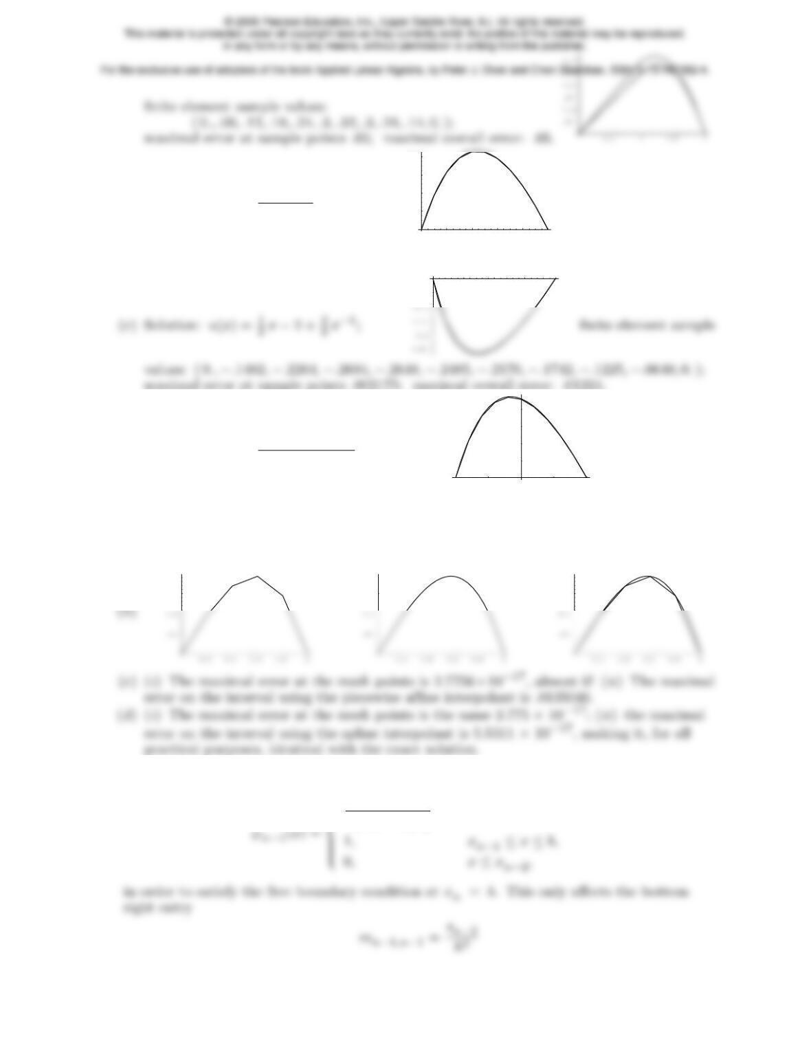
values: ( 0., .03746, .06297, .07844, .08535, .08489, .07801, .06549, .04796, .02598,0.);
maximal error at sample points .00007531; maximal overall error: .001659.
1.5 2 2.5 3
-0.05
maximal error at sample points .002175; maximal overall error: .01224.
(d) Solution: u(x) = e2+ 1 −2e1−x
e2−1−x;
-1 -0.5 0.5 1
0.1
0.2
0.3
0.4
finite element
sample values: ( 0., .2178, .3602, .4407, .4706, .4591, .4136, .3404, .2444, .1298,0.);
maximal error at sample points .003143; maximal overall error: .01120.
♣11.6.3.
(a) The finite element sample values are c= ( 0, .096, .168, .192, .144,0 )T.
0.15
0.15
0.15
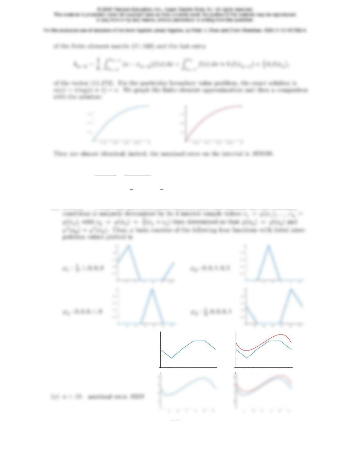
♣11.6.4. The only difference is the last basis function, which should changed to
>
>
>
>
>
<
x−xn−2
xn−1−xn−2
, xn−2≤x≤xn−1,
342
♣11.6.5.
(a)u(x) = x+π ex
1−e2π+π e−x
1−e−2π.
(b) Minimize P[u] = Z2π
0h1
2u′(x)2+1
2u(x)2−xu(x)idx over all C2functions u(x) that
satisfy the boundary conditions u(0) = u(2π), u′(0) = u′(2π).
(c) dim W5= 4 since any piecewise affine function ϕ(x) that satisfies the two boundary
(d)n= 5: maximal error .9435
1234 5 6
1
2
3
4
12 3 4 5 6
1
2
3
4
343
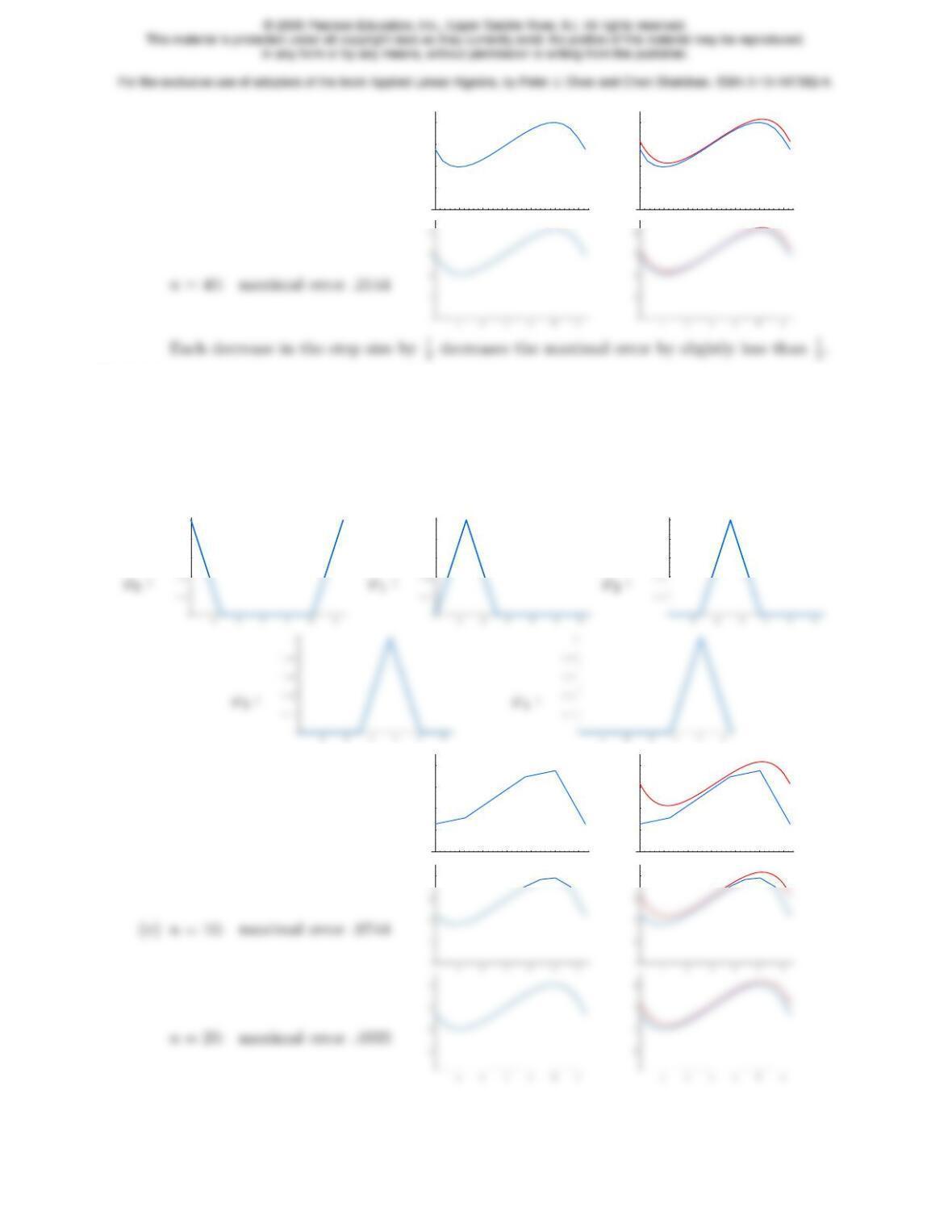
n= 20: maximal error .3792
12 3 4 5 6
1
2
3
4
12 3 4 5 6
1
2
3
4
♣11.6.6.
(c) dim W5= 5, since a piecewise affine function ϕ(x) that satisfies the two boundary con-
ditions is uniquely determined by its values cj=ϕ(xj), j= 0, . . . , 4. A basis consists
of the 5 functions interpolating the values ϕi(xj) = (1, i =j,
0, i 6=j, for 0 ≤i, j < 5, and
ϕi(2π) = ϕi(x5) = ϕi(x0) = ϕi(0). The basis functions are graphed below:
0.6
0.8
1
0.6
0.8
1
0.6
0.8
1
(d)n= 5: maximal error 1.8598
12 3 4 5 6
1
2
3
4
12 3 4 5 6
1
2
3
4
4
4
344
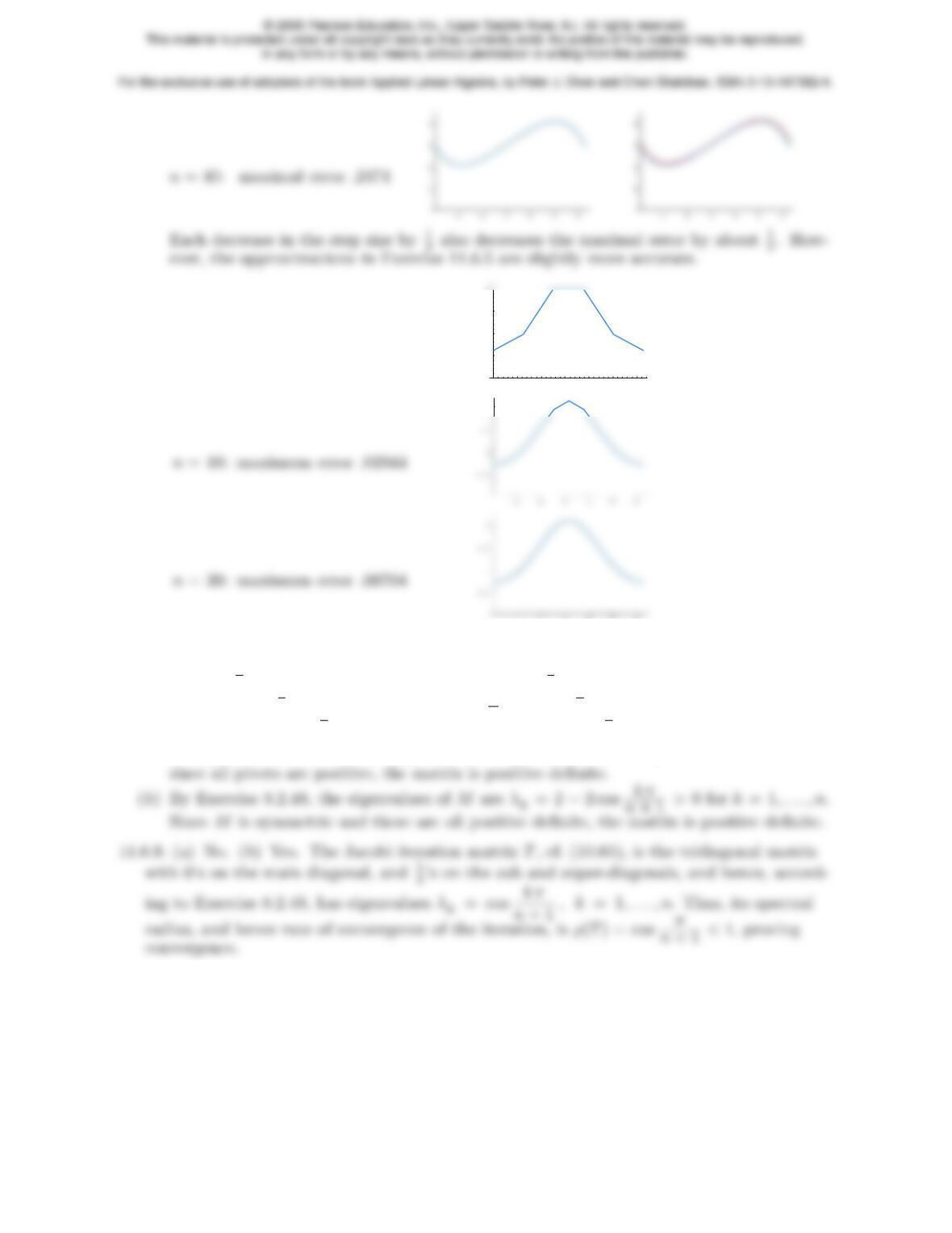
♣11.6.7. n= 5: maximum error .1117
123456
0.5
1
1.5
2
2
12 3 4 5 6
11.6.8.
(a)L=
0
B
B
B
B
B
B
B
B
@
1
−1
21
−2
31
−3
41
......
1
C
C
C
C
C
C
C
C
A
, D =1
h
0
B
B
B
B
B
B
B
B
@
33
24
35
4
...
1
C
C
C
C
C
C
C
C
A
;
♣11.6.10.
(a) A basis for Wnconsists of the n−1 polynomials ϕk(x) = xk(x−1) = xk+1 −xkfor
k= 1, . . . , n −1.
345
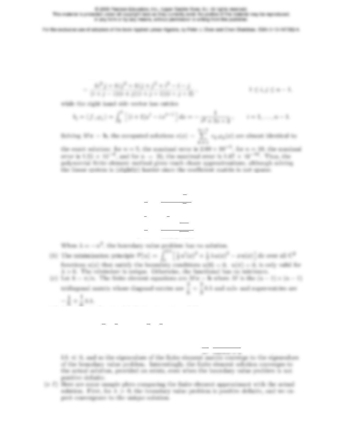
(b) The matrix entries are
mij =hhL[ϕi], L[ϕj]ii =hhϕ′
i, ϕ′
jii
=Z1
0h(i+ 1)xi−ixi−1ih(j+ 1)xj−j xj−1i(x+ 1) dx
♣11.6.11.
(a) There is a unique solution provided λ6=−n2for n= 1,2,3, . . . , namely
u(x) =
8
>
>
>
>
>
>
>
>
>
<
>
>
>
>
>
>
>
>
>
:
x
λ−πsinh √λ x
λsinh √λ π , λ > 0,
1
6π2x−1
6x3, λ = 0,
x
λ−πsin √−λ x
λsin √−λ π ,−n26=λ < 0.
6hλ.
(d) According to Exercise 8.2.48, the eigenvalues of Mare
2
h+2
3hλ + −2
h+1
3hλ !cos k h, k = 1, . . . , n −1.
The finite element system has a solution if and only if the matrix is not singular, which
occurs if and only if 0 is an eigenvalue, and so λ=6
cos k h −1
346
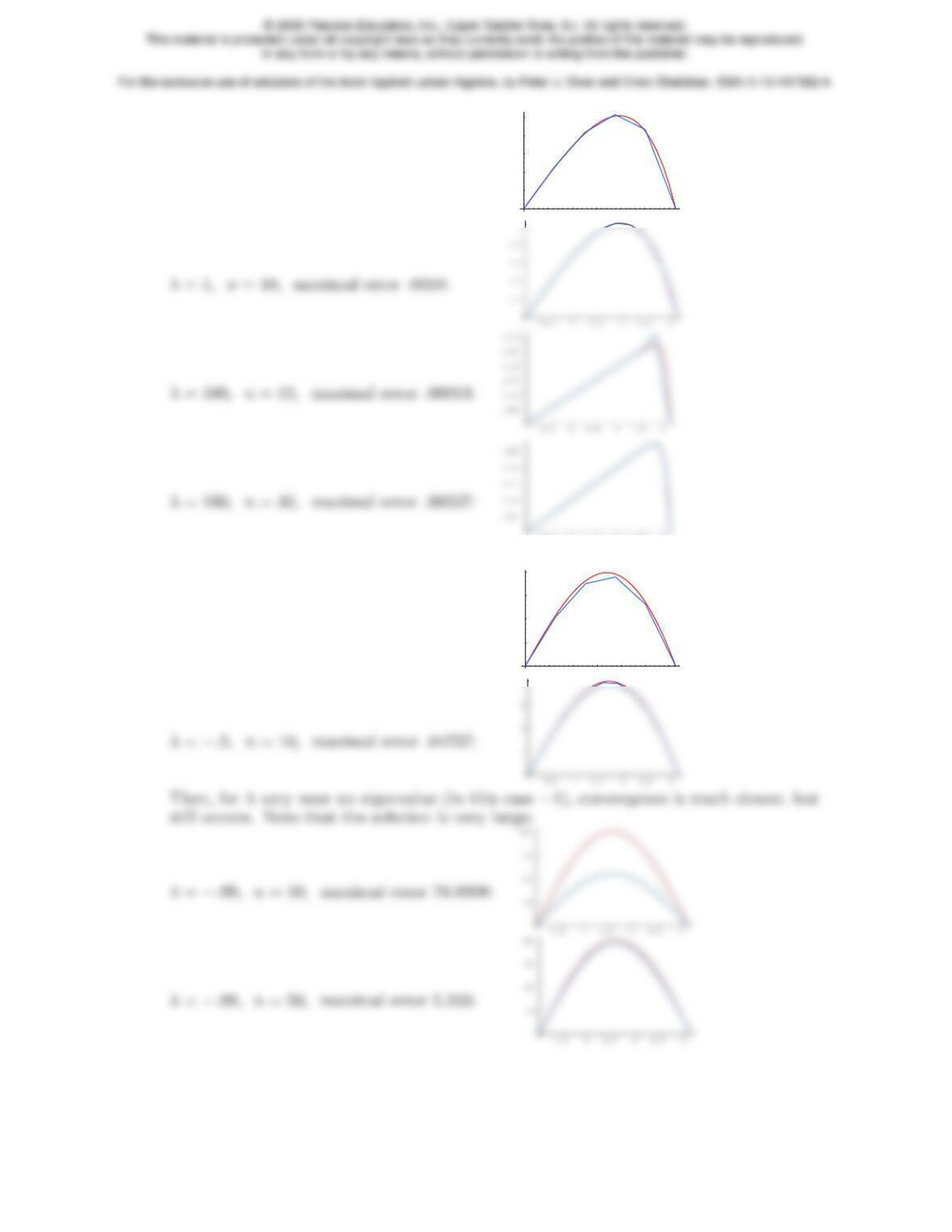
λ= 1, n= 5, maximal error .1062:
0.5 1 1.5 2 2.5 3
0.2
0.4
0.6
0.8
1
0.5 1 1.5 2 2.5 3
Then, for negative λnot near an eigenvalue the convergence rate is simliar:
λ=−.5, n= 5, maximal error .2958:
0.5 1 1.5 2 2.5 3
1
2
3
4
4
347
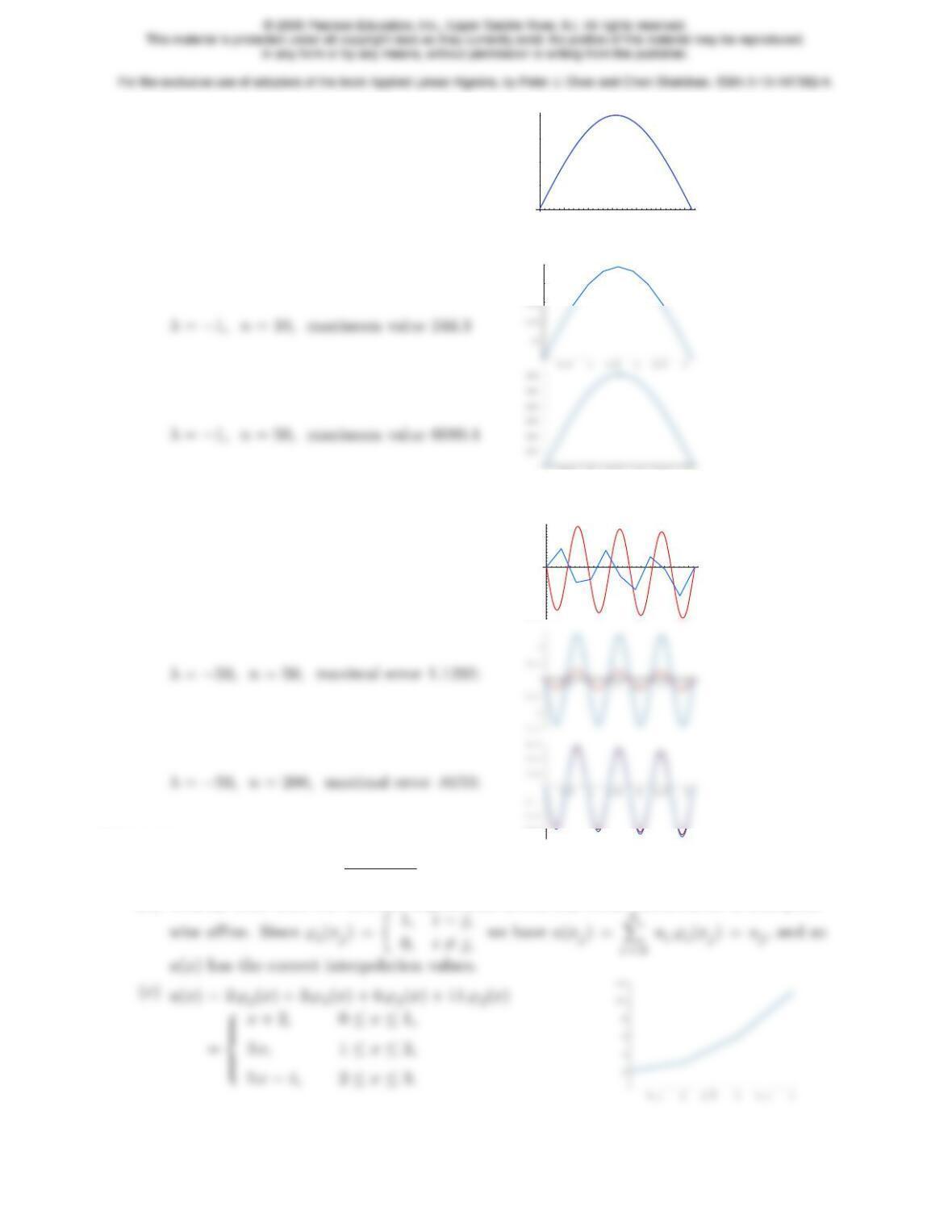
λ=−.99, n= 50, maximal error .4124:
0.5 1 1.5 2 2.5 3
50
100
150
200
On the other hand, when λis an eigenvalue, the finite element solutions don’t converge.
Note the scales on the two graphs:
200
250
0.5 1 1.5 2 2.5 3
The final example shows convergence even for large negative λ. The convergence is slow
because −50 is near an eigenvalue of −49:
λ=−50, n= 10, maximal error .3804:
0.5 1 1.5 2 2.5 3
-0.3
-0.2
-0.1
0.1
0.2
-0.3
♥11.6.12.
(a) We define f(x) = ui+ui+1 −ui
xi+1 −xi
(x−xi) for xi≤x≤xi+1.
(b) Clearly, since each hat function is piecewise affine, any linear combination is also piece-
348
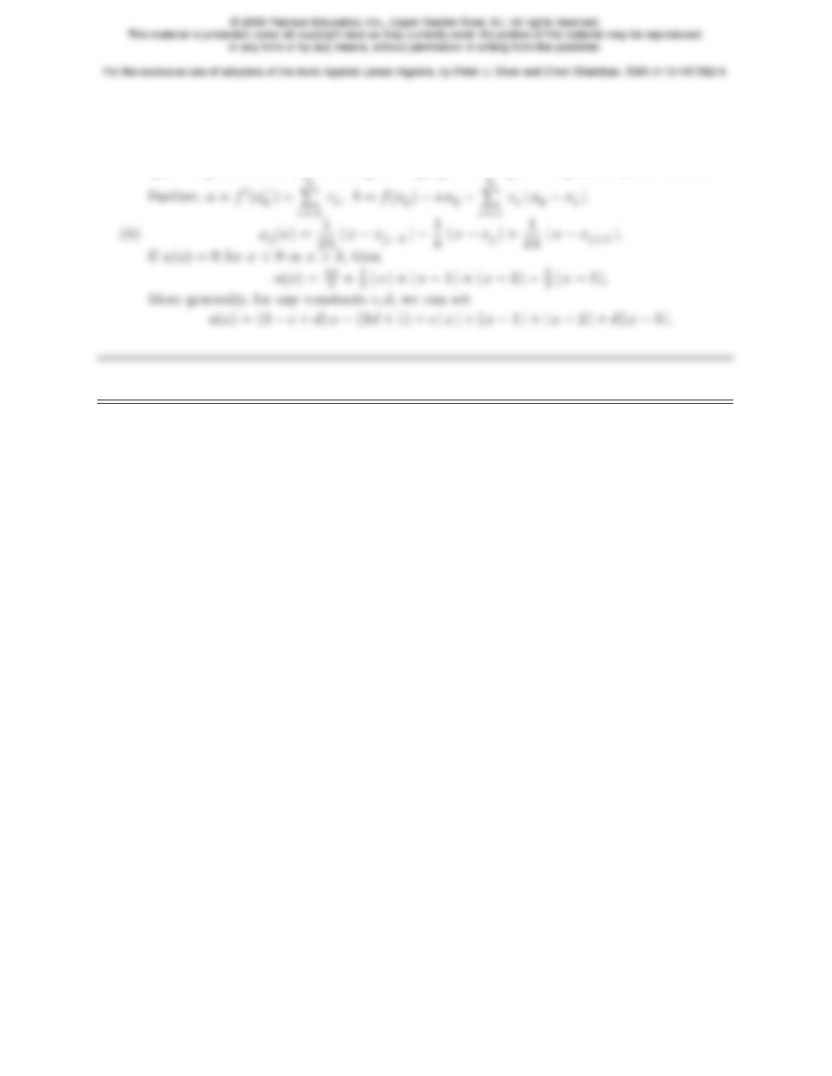
♦11.6.13.
(a) If α(x) is any continuously differentiable function at xj, then α′(x+
j)−α′(x−
j) = 0.
Now, each term in the sum is continuously differentiable at x=xjexcept for αj(x) =
cj|x−xj|, and so f′(x+
j)−f′(x−
j) = α′
j(x+
j)−α′
j(x−
j) = 2cj, proving the formula.
349