Mathematics Chapter 10 That Tis complete with a single dominant

10.4.6. The transition matrix T=0

B

@

02

32

3

1 0 1

3

01

30

1

C

Ais regular because T4=0

B

@

14

27 26

81 26

81

2

949

81 16

27

7

27 2

27 7

81

1

C

A

has all positive entries. She visits branch A 40% of the time, branch B 45% and branch C:

15%.

10.4.9. This is not a regular transition matrix, so we need to analyze the iterative process di-

rectly. The eigenvalues of Aare λ1=λ2= 1 and λ3=1

2, with corresponding eigenvectors

10.4.10. Numbering the vertices from top to bottom and left to right, the transition matrix is

0

B

01

41

4000

1

C

0

B

1

9

2

1

C

10.4.11. Numbering the vertices from top to bottom and left to right, the transition matrix is

0

B

01

41

40000000

1

201

41

600000

1

21

40 0 1

61

40 0 0 0

1

C

0

B

1

18

1

9

1

9

1

C

297

10.4.12. The transition matrix T=

0

B

01

301

300000

1

201

40000

01

30001

3000

1

20 0 0 1

401

20 0

1

C

is not regular. Indeed,

♦10.4.13. The ith column of Tkis u(k)

i=Tkei→vby Theorem 10.40.

10.4.14. In view of Exercise 10.4.13, the limit is 0

B

@

1

31

3

1

31

3

1

31

3

1

C

A.

10.4.15. First, vis a probability vector since the sum of its entries is p

n, . . . , 1

n«T.

10.4.17. z=„1

n, . . . , 1

n«T.

10.4.18. False: 0

B

@

.3.5.2

.3.2.5

.4.3.31

C

Ais a counterexample.

10.4.22. True. If v= ( v1, v2,…,vn)Tis a probability eigenvector, then

n

X

i= 1

vi= 1 and

n

X

j= 1

tij vj=λvifor all i= 1, . . . , n. Summing the latter equations over i, we find

298

♦10.4.24. The ith entry of vis vi=

n

X

j= 1

tij uj. Since each tij ≥0 and uj≥0, the sum vi≥0

also. Moreover,

n

X

vi=

n

X

tij uj=

n

X

uj= 1 because all the column sums of Tare

10.5.1.

10.5.2.

(a)ρ(T) = 2; the iterates diverge: ku(k)k → ∞ at a rate of 2.

10.5.3. (a,b,e,g) are diagonally dominant.

♠10.5.5. (c) Jacobi spectral radius = .547723, so Jacobi converges to the solution

x=8

7= 1.142857, y =19

7= 2.71429;

(d) Jacobi spectral radius = .5, so Jacobi converges to the solution

x=−10

9=−1.1111, y =−13

9=−1.4444, z =2

9=.2222;

(f) Jacobi spectral radius = 1.1180, so Jacobi does not converge.

299

♣10.5.7.

(a)|c|>2.

(b) If c= 0, then D=cI = O, and Jacobi iteration isn’t even defined. Otherwise, T=

−D−1(L+U) is tridiagonal with diagonal entries all 0 and sub- and super-diagonal

entries equal to −1/c. According to Exercise 8.2.48, the eigenvalues are −2

10.5.8. If Au=0, then Du=−(L+U)u, and hence Tu=−D−1(L+U)u=u, proving that

uis a eigenvector for Twith eigenvalue 1. Therefore, ρ(T)≥1, which implies that Tis not

a convergent matrix.

♦10.5.9. If Ais nonsingular, then at least one of the terms in the general determinant expansion

(1.85) is nonzero. If a1,π(1) a2,π(2) ··· an,π(n)6= 0 then each ai,π(i)6= 0. Applying the per-

mutation πto the rows of Awill produce a matrix whose diagonal entries are all nonzero.

10.5.10. Assume, for simplicity, that Tis complete with a single dominant eigenvalue λ1, so

♥10.5.12.

(a)x=0

B

@

7

23

6

23

40

1

C

A=0

B

@

.30435

.26087

1.73913 1

C

A;

300

(c)x(k+1) =0

B

@

0−1

41

2

1

40−1

4

1

C

Ax(k)+0

B

@

−1

2

−1

4

7

1

C

A;

03

64 −1

32

(f)ρ(TJ) = √3

4=.433013,

(g)ρ(TGS ) = 3+√73

64 =.180375, so Gauss–Seidel converges about log ρGS /log ρJ= 2.046

♠10.5.13. (a)x=1

7=.142857, y =−2

7=−.285714; (b)x=−30, y = 48;

(e)x=−1.9172, y =−.339703, z =−2.24204;

(g)x=−.84507, y =−.464789, z =−.450704;

10.5.15.

(a) Solution: u= .7857

.3571 !; spectral radii: ρJ=1

√15 =.2582, ρGS =1

15 =.06667,so

Gauss–Seidel converges exactly twice as fast;

301

(f) Solution: u=0

B

@

0.

.7143

−.1429

−.2857

C

A; spectral radii: ρJ=.4714, ρGS =.3105,so Gauss–Seidel

converges log ρGS /log ρJ= 1.5552 times as fast.

♣10.5.16. (a)|c|>2; (b)c > 1.61804; (c) same answer; (d) Gauss–Seidel converges exactly

twice as fast since ρGS =ρ2

Jfor all values of c.

10.5.19. ρ(TJ) = 0, while ρ(TGS ) = 2. Thus Jacobi converges extremely rapidly, whereas

Gauss–Seidel diverges.

♠10.5.20. Jacobi doesn’t converge because its spectral radius is 3.4441. Gauss–Seidel converges,

but extremely slowly, since its spectral radius is .999958.

♣10.5.23.

(a) If λis an eigenvalue of T= I −A, then µ= 1 −λis an eigenvalue of A, and hence the

eigenvalues of Amust satisfy |1−µ|<1, i.e., they all lie within a distance 1 of 1.

(b) The Gerschgorin disks are

D1={|z−.8| ≤ .2}, D2={|z−1.5| ≤ .3}, D3={|z−1| ≤ .3},

302

♥10.5.24.

(a)u= 1.4

.2!.

(b) The spectral radius is ρJ=.40825 and so it takes about −1/log10 ρJ≈2.57 iterations

to produce each additional decimal place of accuracy.

♣10.5.25. (a)x=.5, y =.75, z =.25, w =.5. (b) To obtain 5 decimal place accuracy,

Jacobi requires 14 iterations, Gauss–Seidel requires 8 iterations. One can get very good

approximations of the spectral radii ρJ=.5, ρGS =.25, by taking ratios of entries of

successive iterates, or the ratio of norms of successive error vectors. (c) The optimal SOR

scheme has ω= 1.0718, and requires 6 iterations to get 5 decimal place accuracy. The SOR

spectral radius is ρSOR =.0718.

♠10.5.27. (a)ρJ=1+√5

4=.809017, ρGS =3+√5

8=.654508; (b) no; (c)ω⋆= 1.25962

and ρ⋆= 1.51315, so SOR with that value of ωdoesn’t converge! However, by numerically

computing the spectral radius of Tω, the optimal value is found to be ω⋆=.874785 (under-

relaxation), with ρ⋆=.125215. (d) The solution is x= (.413793,−.172414, .0689655,

−.0344828)T. Jacobi: predicted 44 iterations; actual 38 iterations. Gauss-Seidel: predicted

22 iterations; actual 19 iterations. Optimal SOR: predicted 5 iterations; actual 5 iterations.

41 iterations, which is about 18 times as fast as Gauss–Seidel.

303

♠10.5.30. The Jacobi and Gauss–Seidel spectral radii are ρJ=√7

3=.881917, ρGS =7

9=

.777778, respectively. It takes 99 Jacobi iterations versus 6 Gauss-Seidel iterations to ob-

tain the solution with 5 decimal place accuracy. Using (10.86) to fix the optimal SOR pa-

rameter ω⋆= 1.35925 with spectral radius ρ⋆=.359246. However, it takes 16 iterations to

obtain the solution with 5 decimal place accuracy, which is significantly slower than Gauss-

Seidel, which converges much faster than it should, owing to the particular right hand side

of the linear system.

♣10.5.32. Using (10.86), the optimal SOR parameter is ω⋆=2

1 + q1−ρ2

J

=2

1 + sin π

n+1

.

For the n= 5 system, ρJ=√3

2, and ω⋆=4

3with ρ⋆=1

3, and the convergence is about 8

times as fast as Jacobi, and 4 times as fast as Gauss–Seidel. For the n= 25 system, ρJ=

.992709, and ω⋆= 1.78486 with ρ⋆=.78486, and the convergence is about 33 times as fast

as Jacobi, and 16.5 times as fast as Gauss–Seidel.

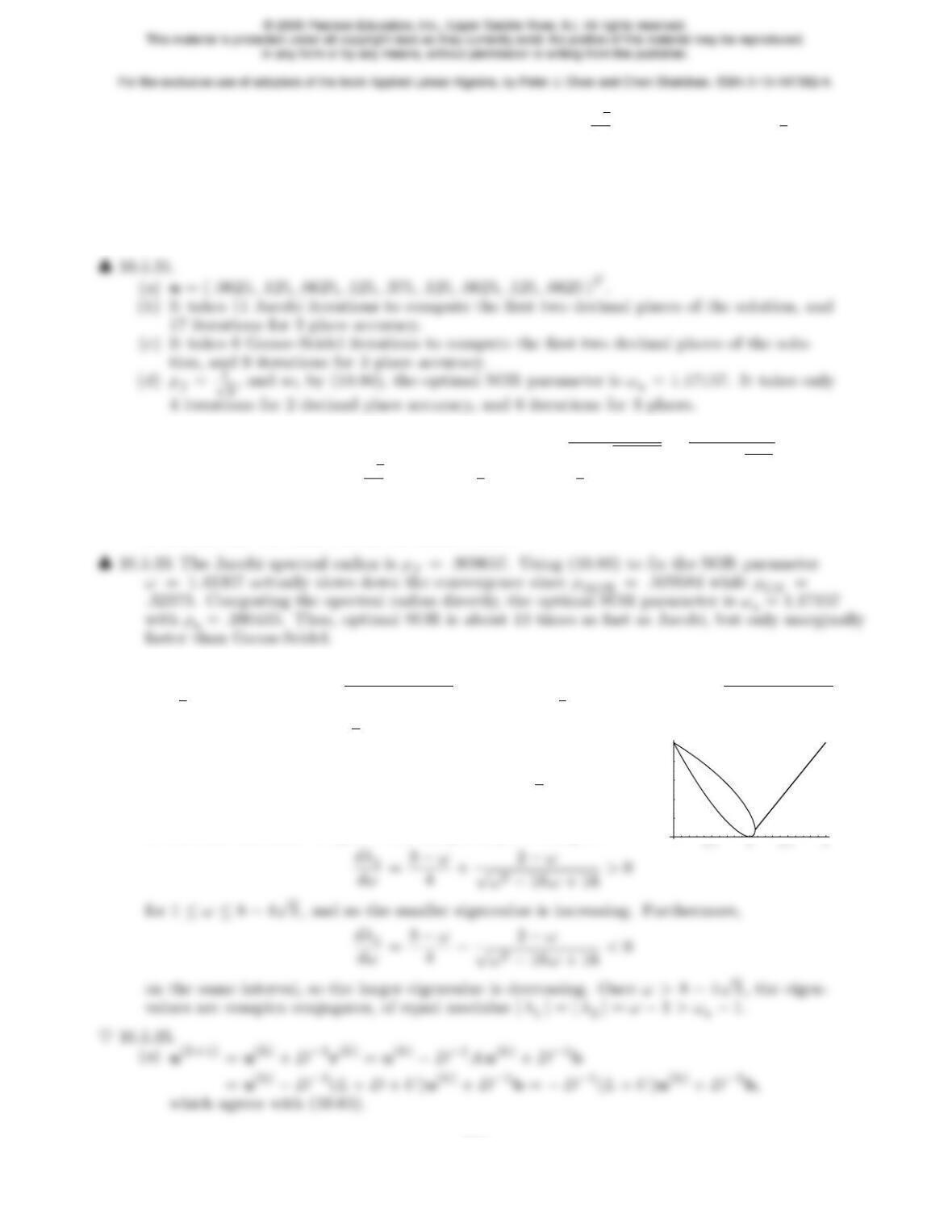
♦10.5.34. The two eigenvalues

λ1=1

8„ω2−8ω+ 8 + ωqω2−16ω+ 16 «, λ2=1

8„ω2−8ω+ 8 −ωqω2−16ω+ 16 «.

are real for 0 ≤ω≤8−4√3 . A graph of the modulus

of the eigenvalues over the range 0 ≤ω≤2 reveals that,

as ωincreases, the smaller eigenvalue is increasing

and the larger decreasing until they meet at 8 −4√3 ;

0.2

0.4

0.6

0.8

1

after this point, both eigenvalues are complex conjugates

of the same modulus. To prove this analytically, we compute

304

(b)u(k+1) =u(k)+ (L+D)−1r(k)=u(k)−(L+D)−1Au(k)+ (L+D)−1b

=u(k)−(L+D)−1(L+D+U)u(k)+ (L+D)−1b

=−(L+D)−1Uu(k)+ (L+D)−1b,

which agrees with (10.71).

(d) If u⋆is the exact solution, so Au⋆=b, then r(k)=A(u⋆−u(k)) and so ku(k)−u⋆k ≤

kA−1k kr(k)k. Thus, if kr(k)kis small, the iterate u(k)is close to the solution u⋆pro-

vided kA−1kis not too large. For instance, if A= 1 0

0.0001 !and b= 1

0!, then

x= 1

100 !has residual r=b−Ax= 0

.001 !, even though xis nowhere near the

exact solution x⋆= 1

0!.

10.5.37.

In each solution, the last ukis the actual solution, with residual rk=f−Kuk=0.

(a)r0= 2

1!,u1= .76923

.38462 !,r1= .07692

−.15385 !,u2= .78571

.35714 !;

(b)r0=0

B

@

1

0

C

A,u1=0

B

@

.5

0

C

A,r1=0

B

@−1

−2

C

A,u2=0

B

@

.51814

−.72539

C

A,

305

0

−.8

−.125

♣10.5.38. Remarkably, after only two iterations, the method finds the exact solution: u3=u⋆=

(.0625, .125, .0625, .125, .375, .125, .0625, .125, .0625 )T, and hence the convergence is dra-

matically faster than the other iterative methods.

♣10.5.39. (a)n= 5: b= ( 2.28333,1.45,1.09286, .884524, .745635 )T;

n= 10: b= ( 2.92897,2.01988,1.60321,1.3468,1.16823,1.0349, .930729, .846695, .777251, .718771 )T;

n= 30: b= (3.99499,3.02725,2.5585,2.25546,2.03488,1.86345,1.72456,1.60873,1.51004,1.42457,

1.34957,1.28306,1.22353,1.16986,1.12116,1.07672,1.03596, .998411, .963689, .931466,

.901466, .873454, .847231, .82262, .799472, .777654, .75705, .737556, .719084, .70155)T;

(b) For regular Gaussian Elimination, using standard arithmetic in Mathematica, the

10.5.41. False. For example, consider the homogeneous system Ku=0where K= .0001 0

0 1 !,

with solution u⋆=0. The residual for u= 1

10.5.42. Referring to the pseudocode program in the text, at each step to compute

rk=f−Kukrequires n2multiplications and n2additions;

krkk2requires nmultiplications and n−1 additions;

♦10.5.43. tk=krkk2

rT

kKrk

=uT

kK2uk−2fTKuk+kfk2

uT

kK3uk−2fTK2uk+fTKf.

♠10.6.1. In all cases, we use the normalized version (10.101) starting with u(0) =e1; the answers

are correct to 4 decimal places.

(a) After 17 iterations, λ= 2.00002, u= ( −.55470, .83205 )T;

♠10.6.2.

For n= 10, it takes 159 iterations to obtain λ1= 3.9189 = 2 + 2 cos 1

6πto 4 decimal places.

for n= 20, it takes 510 iterations to obtain λ1= 3.9776 = 2 + 2 cos 1

21 πto 4 decimal places.

for n= 50, it takes 2392 iterations to obtain λ1= 3.9962 = 2 + 2 cos 1

51 πto 4 decimal

places.

♠10.6.3. In each case, to find the dominant singular value of a matrix A, we apply the power

307

10.6.4. Since v(k)→λk

1v1as k→ ∞,

♦10.6.5.

(a) If Av=λvthen A−1v=1

λv, and so vis also the eigenvector of A−1.

(b) If λ1, . . . , λnare the eigenvalues of A, with |λ1|>|λ2|>···>|λn|>0 (recalling that

0 cannot be an eigenvalue if Ais nonsingular), then 1

λ1

,…, 1

λn

are the eigenvalues of

♠10.6.6.

(a) After 15 iterations, we obtain λ=.99998, u= ( .70711,−.70710 )T;

(b) after 24 iterations, we obtain λ=−1.99991, u= ( −.55469,−.83206 )T;

(h) after 16 iterations, we obtain λ= 2.00006, u= ( .500015,−.50000, .499985,−.50000 )T.

♦10.6.7.

(a) According to Exercises 8.2.19, 8.2.24, if Ahas eigenvalues λ1, . . . , λn, then (A−µI )−1

♠10.6.8.

(a) After 11 iterations, we obtain ν⋆= 2.00002, so λ⋆= 1.0000, u= ( .70711,−.70710 )T;

308

(b) after 27 iterations, we obtain ν⋆=−.40003, so λ⋆=−1.9998, u= ( .55468, .83207 )T;

(c) after 10 iterations, we obtain ν⋆= 2.00000, so λ⋆= 1.00000,

u= ( .40825, .81650, .40825 )T;

(d) after 7 iterations, we obtain ν⋆=−5.07037, so λ⋆=.30278,

u= ( −.35355, .46060,−.81415 )T;

♠10.6.9.

(i) First, compute the dominant eigenvalue λ1and eigenvector v1using the power method.

Then set B=A−λ1v1bT, where bis any vector such that b·v1= 1, e.g., b=

v1/kv1k2. According to Exercise 8.2.52, Bhas eigenvalues 0, λ2, . . . , λn, and corre-

sponding eigenvectors v1and wj=vj−cjv1, where cj=b·vj/λjfor j≥1. Thus,

(b) Using λ1=−3.,v1= ( .70711, .70711 )T, the deﬂated matrix is B= −3.5 3.5

−1.5 1.5!; it

takes 3 iterations to produce λ2=−2.00000.

(c) Using λ1= 4.,v1= ( .57737,−.57735, .57735 )T, the deﬂated matrix is

B=0

B

@

1.66667 .333333 −1.33333

.333333 .666667 .333333

−1.33333 .333333 1.66667 1

C

A; it takes 11 iterations to produce λ2= 2.99999.

309

is B=0

B

@

1.5−.19098 −.80902 .5000

−.19098 .69098 .30902 −.80902

−.80902 .30902 .69098 −.19098

.5000 −.80902 −.19098 1.5000

C

A; it takes 18 iterations to produce

λ2= 2.61801.

10.6.10. That Ais a singular matrix and 0 is an eigenvalue. The corresponding eigenvectors are

10.6.11.

(a) Eigenvalues: 6.7016, .2984; eigenvectors: .3310

.9436 !, .9436

−.3310 !.

(b) Eigenvalues: 5.4142,2.5858; eigenvectors: −.3827

.9239 !, .9239

.3827 !.

10.6.12. The iterates converge to the diagonal matrix An→0

B

@

0 9 0

0 0 3 1

C

A. The eigenvalues ap-

10.6.13.

(a) Eigenvalues: 2,1; eigenvectors: −2

3!, −1

1!.

310

(b) Eigenvalues: 1.2087,5.7913; eigenvectors: −.9669

.2550 !, −.6205

−.7842 !.

(c) Eigenvalues: 3.5842,−2.2899,1.7057;

eigenvectors: 0

B

@−.4466

−.7076

C

A,0

B

@

.1953

−.8380

C

A,0

B

@

.7491

−.2204

C

A.

10.6.14. Yes. After 10 iterations, one finds

R10 =0

B

@

2.0011 1.4154 4.8983

0.9999 −.0004

0 0 .9995 1

C

A, S10 =0

B

@−.5773 .4084 .7071

−.5774 .4082 −.7071

−.5774 −.8165 .0002 1

C

A,

so the diagonal entries of R10 give the eigenvalues correct to 3 decimal places, and the

columns of S10 are similar approximations to the orthonormal eigenvector basis.

♦10.6.17.

(a) By induction, if Ak=QkRk=RT

kQT

k=AT

k, then, since Qkis orthogonal,

AT

k+1 = (RkQk)T=QT

kRT

k=QT

kRT

kQT

kQk=QT

kQkRkQk=RkQk=Ak+1,

(b) The result does not hold if Ais only tridiagonal and not symmetric. For example, when

311

10.6.18.

(a)H=0

B

@

1 0 0

0−.9615 .2747

0.2747 .9615 1

C

A, T =H AH =0

B

@

8.0000 7.2801 0

7.2801 20.0189 3.5660

0 3.5660 4.9811 1

C

A.

(b)

(c)

H1=0

B

@

1 0 0 0

0 0 .7071 −.7071

0.7071 .5000 .5000

0−.7071 .5000 .5000

1

C

A, T1=H1AH1=0

B

@

4.0000 −1.4142 0 0

−1.4142 2.5000 .1464 −.8536

0.1464 1.0429 .7500

0−.8536 .7500 2.4571

1

C

A,

♠10.6.19.

(a) Eigenvalues: 24,6,3; (b) eigenvalues: 7.6180,7.5414,5.3820,1.4586;

(c) eigenvalues: 4.9354,3.0000,1.5374, .5272.

♠10.6.20. The singular values are the square roots of the non-zero eigenvalues of

Applying the QR algorithm to the final tridiagonal matrix, the eigenvalues are found to be

14.4131, 7.66204,2.92482,0, and so the singular values of the original matrix are

3.79646,2.76804,1.71021.

312

(b)

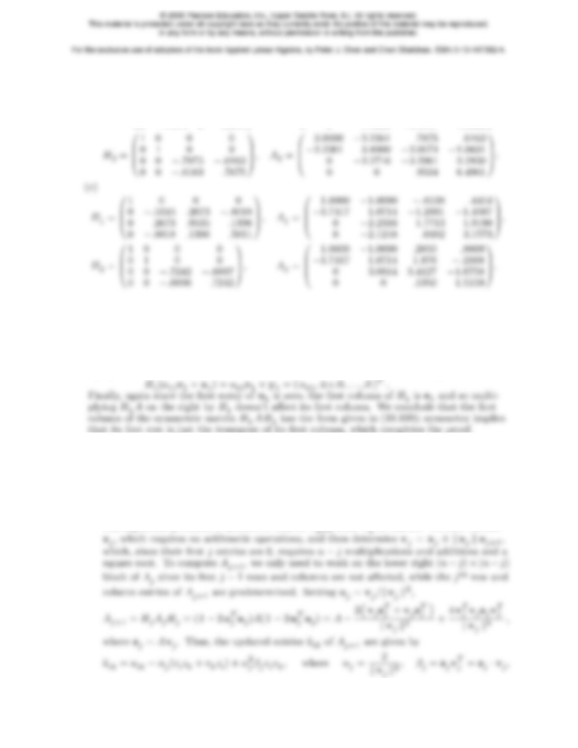
H1=0

B

@

1 0 0 0

0−.8944 0 −.4472

0 0 1 0

0−.4472 0 .8944

1

C

A, A1=0

B

@

3.0000 −2.2361 −1.0000 0

−2.2361 3.8000 2.2361 .4000

0 1.7889 2.0000 −5.8138

0 1.4000 −4.4721 1.2000

1

C

A,

♠10.6.22.

(a) Eigenvalues: 4.51056,2.74823,−2.25879,

(b) eigenvalues: 7., 5.74606,−4.03877,1.29271,

(c) eigenvalues: 4.96894,2.31549,−1.70869,1.42426.

10.6.23. First, by Lemma 5.28, H1x1=y1. Furthermore, since the first entry of u1is zero,

uT

1e1= 0, and so He1= ( I −2u1uT

1)e1=e1. Thus, the first column of H1Ais

10.6.24. Since T=H−1AH where H=H1H2···Hnis the product of the Householder reﬂec-

tions, Av=λvif and only if Tw=λwwhere w=H−1vis the corresponding eigenvector

of the tridiagonalized matrix. Thus, to recover the eigenvectors of Awe need to multiply

v=Hw=H1H2···Hnw.

♦10.6.25.

(a) Starting with a symmetric matrix A=A1, for each j= 1,…,n−1, the tridiagonaliza-

tion algorithm produces a symmetric matrix Aj+1 from Ajas follows. We first extract

313

(b) First, to factor a tridiagonal A=QR using the pseudocode program on page 242, we

note that at the beginning of the jth step, for j < n, the last n−j−1 entries of the

jth column and the last n−j−2 entries of the (j+ 1)st column are zero, while columns

j+ 2, . . . , n are still in tridaigonal form. Thus, to compute rjj requires j+ 1 multiplica-

(c) Much faster: Once the matrix is tridiagonalized, each iteration requires 5

2n2versus n3

multiplications and 3

2n2versus n3additions, as found in Exercise 5.3.31. Moreover, by

part (a), the initial triadiagonalization only requires the effort of about 1 1

2QR steps.

10.6.26.

Tridiagonalization

start

set R=A

for j= 1 to n−2

314