Mathematics Chapter 1 Running Gaussian Elimination with pivoting

1.7.19. (a)x=−220., y = 26, z =.91; (b)x=−190., y = 24, z =.84; (c)x=−210,

y= 26, z = 1.(d) The exact solution is x=−213.658, y = 25.6537, z =.858586.

Full pivoting is the most accurate. Interestingly, partial pivoting fares a little worse than

regular elimination.

1.7.20. (a)0

B

@

6

5

−13

5

−9

5

1

C

A=0

B

@

1.2

−2.6

−1.81

C

A, (b)0

B

@

−1

4

−5

4

1

8

1

C

A

, (c)0

B

@

0

1

0

1

C

A, (d)0

B

@

−32

35

−19

35

−12

35

−76

1

C

A

=0

B

@

−.9143

−.5429

−.3429

−2.1714

1

C

A.

1.7.22. The results are the same.

♠1.7.23.

Gaussian Elimination With Full Pivoting

start

for i= 1 to n

set σ(i) = τ(i) = i

next i

for j= 1 to n

if mσ(i),j = 0 for all i≥j, stop; print “Ais singular”

32

♠1.7.24. We let x∈Rnbe generated using a random number generator, compute b=Hnxand

then solve Hny=bfor y. The error is e=x−yand we use e⋆= max |ei|as a measure of

the overall error. Using Matlab, running Gaussian Elimination with pivoting:

n10 20 50 100

e⋆.00097711 35.5111 318.3845 1771.1

♠1.7.25.

(a)H−1

3=0

B

@

9−360 30

−36 192 −180

30 −180 180 1

C

A,

(b) The same results are obtained when using ﬂoating point arithmetic in either Mathe-

matica or Matlab.

(c) The product f

K10H10, where f

K10 is the computed inverse, is fairly close to the 10 ×10

identity matrix; the largest error is .0000801892 in Mathematica or .000036472 in

1.8.1.

(a) Unique solution: (−1

2,−3

4)T;

For the exclusive use of adopters of the book Applied Linear Algebra, by Peter J. Olver and Cheri Shakiban. ISBN 0-13-147382-4.

1.8.2. (a) Incompatible; (b) incompatible; (c) (1,0)T; (d) (1 + 3 x2−2x3, x2, x3)T, where x2

and x3are arbitrary; (e) (−15

2,23,−10)T; (f) (−5−3x4,19 −4x4,−6−2x4, x4)T, where

x4is arbitrary; (g) incompatible.

1.8.4. (i)a6=band b6= 0; (ii)b= 0, a 6=−2; (iii)a=b6= 0, or a=−2 and b= 0.

1.8.6.

1.8.7. (a) 2, (b) 1, (c) 2, (d) 3, (e) 1, (f) 1, (g) 2, (h) 2, (i) 3.

1.8.8.

(a) 1 1

1−2!= 1 0

1 1 ! 1 1

0−3!,

(b) 2 1 3

−2−1−3!= 1 0

−1 1 ! 2 1 3

000!,

(f) ( 0 −1 2 5 ) = ( 1 )( 0 −1 2 5 ),

(g)0

B

@

0 1 0 0

1 0 0 0

0 0 1 0

0 0 0 1

1

C

A0

B

@

0−3

4−1

1 2

−1−5

1

C

A=0

B

@

1 0 0 0

0 1 0 0

1

4−3

41 0

1

C

A0

B

@

1 2

0 7

0 0

1

C

A,

1.8.9. (a)

y= 0,

z= 0.

(b)

y+z= 0,

x−z= 1.

(c)

y+z= 0,

x−z= 0.

34

1.8.11.

(a)x2+y2= 1, x2−y2= 2;

1.8.12. That variable does not appear anywhere in the system, and is automatically free (al-

though it doesn’t enter into any of the formulas, and so is, in a sense, irrelevant).

1.8.13. True. For example, take a matrix in row echelon form with rpivots, e.g., the matrix A

with aii = 1 for i= 1, . . . , r, and all other entries equal to 0.

1.8.14. Both false. The zero matrix has no pivots, and hence has rank 0.

♥1.8.15.

(a) Each row of A=v wTis a scalar multiple, namely viw, of the vector w. If necessary,

we use a row interchange to ensure that the first row is non-zero. We then subtract the

1.8.16. 1.

1.8.17. 2.

1.8.18. Example: A= 1 0

0 0 !, B = 0 1

0 0 !so AB = 0 1

0 0 !has rank 1, but B A = 0 0

0 0 !

has rank 0.

♦1.8.19.

(a) Under elementary row operations, the reduced form of Cwill be “U Z ”where Uis the

♦1.8.20. By Proposition 1.39, Acan be reduced to row echelon form Uby a sequence of elemen-

tary row operations. Therefore, as in the proof of the LU decomposition, A=E1E2· · · ENU

where E−1

1, . . . , E−1

Nare the elementary matrices representing the row operations. If Ais

singular, then U=Zmust have at least one all zero row.

35

♦1.8.21. After row operations, the augmented matrix becomes N=“U|c”where the r= rank A

nonzero rows of Ucontain the pivots of A. If the system is compatible, then the last m−r

entries of care all zero, and hence Nis itself a row echelon matrix with rnonzero rows and

1.8.22. (a)x=z, y =z, where zis arbitrary; (b)x=−2

3z, y =7

9z, where zis arbitrary;

1.8.23. (a)“1

3y, y ”T, where yis arbitrary; (b)“−6

5z, 8

5z, z ”T, where zis arbitrary;

1.8.24. If Uhas only nonzero entries on the diagonal, it must be nonsingular, and so the only

solution is x=0. On the other hand, if there is a diagonal zero entry, then Ucannot have

npivots, and so must be singular, and the system will admit nontrivial solutions.

1.8.25. For the homogeneous case x1=x3,x2= 0, where x3is arbitrary. For the inhomoge-

1.8.26. For the homogeneous case x1=−1

6x3−1

6x4,x2=−2

3x3+4

3x4, where x3and x4

are arbitrary. For the inhomogeneous case x1=−1

6x3−1

6x4+1

3a+1

6b,x2=−2

3x3+

4

3x4+1

3a+1

6b, where x3and x4are arbitrary. The dependence on the free variable x3is

the same as in the homogeneous case.

1.8.27. (a)k= 2 or k=−2; (b)k= 0 or k=1

2; (c)k= 1.

1.9.1.

(a) Regular matrix, reduces to upper triangular form U= 2−1

0 1 !, so determinant is 2;

36

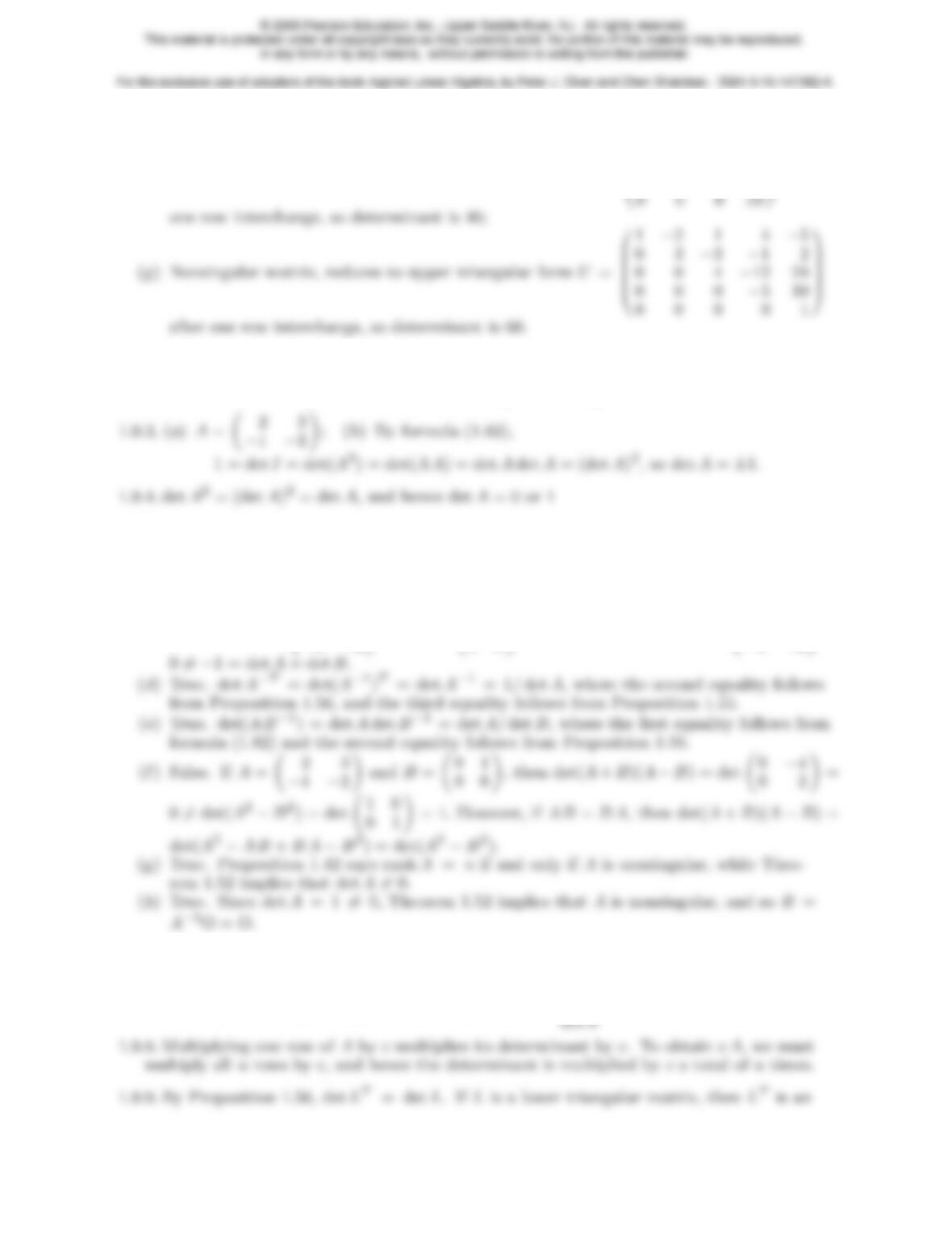
(e) Upper triangular matrix, so the determinant is a product of diagonal entries: −180;

(f) Nonsingular matrix, reduces to upper triangular form U=0

B

@

1−2 1 4

0 2 −1−7

0 0 −2−8

1

C

Aafter

1.9.2. det A=−2, det B=−11 and det A B = det 0

B

@

5 4 4

1 5 1

−2 10 0 1

C

A= 22.

1.9.5.

(a) True. By Theorem 1.52, Ais nonsingular, so, by Theorem 1.18, A−1exists

(b) False. For A= 2 3

−1−2!, we have 2 det A=−2 and det 2 A=−4. In general,

det(2A) = 2ndet A.

(c) False. For A= 2 3

−1−2!and B= 0 1

0 0 !, we have det(A+B) = det 2 4

−1−2!=

1.9.6. Never — its determinant is always zero.

1.9.7. By (1.82, 83) and commutativity of numeric multiplication,

det B= det(S−1AS) = det S−1det Adet S=1

37

upper triangular matrix. By Theorem 1.50, det LTis the product of its diagonal entries

which are the same as the diagonal entries of L.

1.9.10. (a) See Exercise 1.9.8. (b) If nis odd, det(−A) = −det A. On the other hand, if

AT=−A, then det A= det AT=−det A, and hence det A= 0. (c)A= 0 1

−1 0 !.

♦1.9.11. We have

det a b

c+k a d +k b !=ad +a k b −b c −bk a =ad −b c = det a b

c d !,

0d!=ad −b0 = ad.

♦1.9.12.

(a) The product formula holds if Ais an elementary matrix; this is a consequence of the

determinant axioms coupled with the fact that elementary matrices are obtained by ap-

plying the corresponding row operation to the identity matrix, with det I = 1.

1.9.13. Indeed, by (1.82), det Adet A−1= det(AA−1) = det I = 1.

♦1.9.14. Exercise 1.6.28 implies that, if Ais regular, so is AT, and they both have the same piv-

ots. Since the determinant of a regular matrix is the product of the pivots, this implies

1.9.15.

B

a11 a12 a13 a14

a21 a22 a23 a24

1

C

38

♦1.9.16.

(i) Suppose Bis obtained from Aby adding ctimes row kto row l, so

bij =8

<

:

alj +caij , i =l,

aij , i 6=l. Thus, each summand in the determinantal formula for

det Bsplits into two terms, and we find that det B= det A+cdet C, where Cis the

matrix obtained from Aby replacing row lby row k. But rows kand lof Care identi-

cal, and so, by axiom (ii), if we interchange the two rows det C=−det C= 0. Thus,

det B= det A.

♦1.9.17. If Uis nonsingular, then, by Gauss–Jordan elimination, it can be reduced to the iden-

tity matrix by elementary row operations of types #1 and #3. Each operation of type #1

♦1.9.18. The determinant of an elementary matrix of type #2 is −1, whereas all elementary ma-

trices of type #1 have determinant +1, and hence so does any product thereof.

♥1.9.19.

(a) Since Ais regular, a6= 0 and ad −b c 6= 0. Subtracting c/a times the first from from the

second row reduces Ato the upper triangular matrix a b

0d+b(−c/a)!, and its pivots

are aand d−bc

a=ad −b c

a=det A

a.

♥1.9.20. (a–c) Applying an elementary column operation to a matrix Ais the same as apply-

ing the elementary row operation to its transpose ATand then taking the transpose of the

result. Moreover, Proposition 1.56 implies that taking the transpose does not affect the de-

39

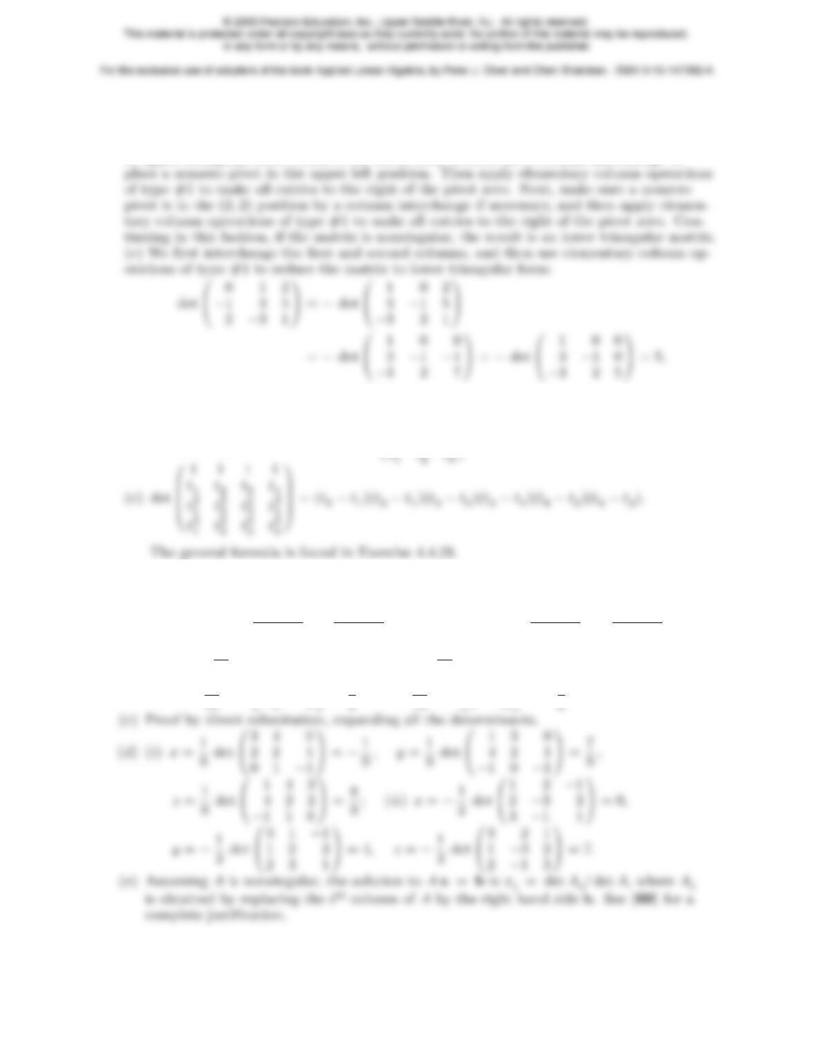
terminant, and so any elementary column operation has exactly the same effect as the cor-

responding elementary row operation.

(d) Apply the transposed version of the elementary row operations required to reduce AT

to upper triangular form. Thus, if the (1,1) entry is zero, use a column interchange to

♦1.9.21. Using the LU factorizations established in Exercise 1.3.25:

(a) det 1 1

t1t2!=t2−t1, (b) det 0

B

@

1 1 1

t1t2t3

1

C

A= (t2−t1)(t3−t1)(t3−t2),

♥1.9.22.

(a) By direct substitution:

ax +b y =apd −b q

ad −b c +baq −p c

ad −b c =p, cx +d y =cpd −b q

ad −b c +daq −p c

ad −b c =q.

(b) (i)x=−1

10 det 13 3

0 2 !=−2.6, y =−1

10 det 1 13

4 0 != 5.2;

(ii)x=1

−2 6 !=5

3−2!=−7

40

♦1.9.23.

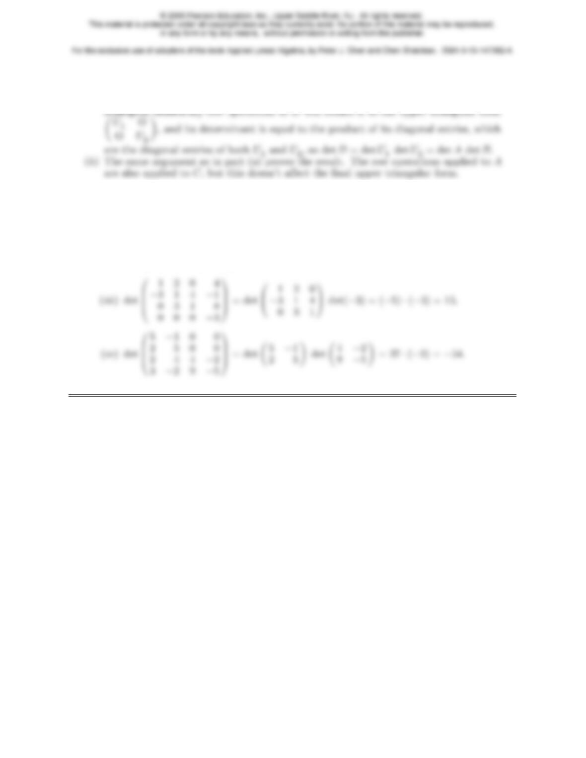
(a) We can individually reduce Aand Bto upper triangular forms U1and U2with the

determinants equal to the products of their respective diagonal entries. Applying the

(c) (i) det 0

B

@

3 2 −2

0 4 −5

0 3 7 1

C

A= det(3) det 4−5

3 7 != 3 ·43 = 129,

(ii) det 0

B

@

1 2 −2 5

−3 1 0 −5

0 0 1 3

0 0 2 −2

1

C

A= det 1 2

−3 1 !det 1 3

2−2!= 7 ·(−8) = −56,

41