
Chapter Fifteen: Testing for Differences Between Groups and for Predictive Relationships 408
Chapter 15
Testing for Differences between
Groups and for Predictive Relationships
AT-A-GLANCE
I. Introduction
II. What Is the Appropriate Test Statistic?
III. Cross-Tabulation Tables: The 2 Test for Goodness-of-Fit
IV. The t-Test for Comparing Two Means
A. Independent samples t-test
B. Independent samples t-test calculation
C. Practically speaking
D. Paired-samples t-test
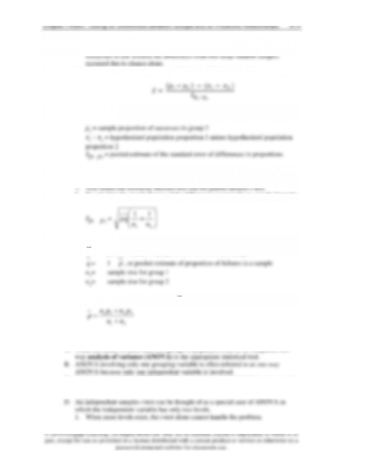
E. The Z-test for comparing two proportions
V. One-Way Analysis of Variance (ANOVA)
A. Simple illustration of ANOVA
B. Partitioning variance in ANOVA
1. Total variability
3. Within-group error
C. The F-Test
2. A different but equivalent representation
D. Practically speaking
VI. Statistical Software
VII. General Linear Model
A. GLM equation
B. Regression analysis
1. Interpreting multiple regression analysis
3. Steps in interpreting a multiple regression model
LEARNING OUTCOMES
2. Compute a χ2 statistic for cross-tab results.
3. Use a t-test to compare a difference between two means.

Chapter Fifteen: Testing for Differences Between Groups and for Predictive Relationships 410
Students are then taken step-by-step through the process of calculating an independent t-test
in both SPSS and JMP.
➢ Is the Price Right?
$30.50 when the wine is French but only $23.53 when they believe it is from Oregon. In
addition, the interaction between origin and the presentation of information is significant. As
a decision maker for a wine company, how could you use this information?
TIPS OF THE TRADE
➢ Cross-tabulations are widely applied in market research reports and presentations.
▪ Cross-tabs can be very useful in big data analysis exploring data for useful
relationships
▪ Cross-tabulations are appropriate for research questions involving predictions of
categorical dependent variables using categorical independent variables.
➢ A t-test can be used to compare means.
▪ An independent samples t-test predicts a continuous (interval or ratio) dependent
variable with a categorical (nominal or ordinal) independent (grouping) variable.
➢ A one-way ANOVA extends the concept of an independent samples t-test to more than two
groups.
Chapter Fifteen: Testing for Differences Between Groups and for Predictive Relationships 411
OUTLINE
I. INTRODUCTION
A. A surprising number of inferences involve two variables.
B. The automated search for relationships between two variables provides the backbone
for automated big data searchers.
II. WHAT IS THE APPROPRIATE TEST STATISTIC?
1. How many independent variables (IV) and dependent variables (DV) are
involved in the analysis?
2. What is the scale level of the independent and dependent variables involved in
the analysis?
E. Exhibit 15.2 provides a useful guide in choosing a test.
III. CROSS-TABULATION TABLES: THE 2 TEST FOR GOODNESS-OF-FIT
A. One of the most widely used and simplest techniques for describing sets of
relationships is the cross-tabulation.
B. A cross-tabulation, or contingency table, is a joint frequency distribution of
observations on two or more nominal or ordinal variables.
C. The 2 distribution provides a means for testing the statistical significance of
contingency tables.
F. The test allows us to conduct tests for significance in the analysis of the R C
contingency table (where R = row and C = column).
𝐸𝑖𝑗 = 𝑅𝑖𝐶𝑗
𝑛
© 2016 Cengage Learning. All Rights Reserved. May not be scanned, copied or duplicated, in whole or in
part, except for use as permitted in a license distributed with a certain product or service or otherwise on a
password-protected website for classroom use.
1. Examine the statistical significance of the observed contingency table.
2. Examine whether the differences between the observed and expected values are
consistent with the hypothesized prediction.
IV. THE t-TEST FOR COMPARING TWO MEANS
A. A t-test is appropriate when a researcher needs to compare means for a variable
grouped into two categories based on some less-than interval variable.
B. One way to think about this is as testing the way a dichotomous (two levels)
independent variable is associated with changes in a continuous dependent variable.
C. Independent Samples t-test
1. Most typically, the researcher will apply the independent samples t-test which
2. This test assumes the two samples are drawn from normal distributions and that
the variances of the two populations are approximately equal (homoscedasticity).
D. Independent Samples t-test Calculation
2. The null hypothesis is normally stated as:
𝜇1= 𝜇2, which is equivalent to 𝜇1− 𝜇2= 0
3. However, since this is inferential statistics, we test the idea by comparing two
21 XX −
4. Thus, the t-value is a ratio with information about the differences between means
6. A pooled estimate of the standard error is a better estimate of the standard
error than one based on the variance from either sample.
7. A higher t-value is associated with a lower p-value, and as the t gets higher and
the p-value gets lower, the researcher has more confidence that the means are
truly different.
F. Practically Speaking
2. Exhibit 15.3 displays a typical t-test printout.
3. These particular results examine the following research question: Does religion
relate to price sensitivity in restaurants?
4. Because no direction of the relationship is stated (no hypothesis is offered), a
© 2016 Cengage Learning. All Rights Reserved. May not be scanned, copied or duplicated, in whole or in
part, except for use as permitted in a license distributed with a certain product or service or otherwise on a
password-protected website for classroom use.
6. Basic steps:
a. Examine the difference in means to find the “direction” of any difference.
b. Compute or locate the computed t-test value.
c. Find the p-value associated with this t and the corresponding degrees of
freedom.
d. The difference can also be examined using the 95 percent confidence
interval, and if the interval does not include 0, we lack sufficient confidence
that the true difference between the population mean is 0.
e. Note:
i. Strictly speaking, the t-test assumes that the two population variances are
equal – a slightly more complicated formula exists which will compute
the t-statistic assuming they are not equal, and SPSS provides both
results when an independent samples t-test is performed.
ii. Even though the means appear to be not so close to each other, the
statistical conclusion could be that they are the same due to the variance
because the t–statistic is a function of the standard error, which is a
function of the standard deviation.
iii. As samples get larger, the t–test and Z-test will tend to yield the same
result.
(a) A t-test can be used with large samples.
G. Paired Samples t-Test
1. A paired samples t-test is appropriate when means that need to be compared are
not from independent samples (i.e., the same respondent is measured twice).
E. THE Z-TEST FOR COMPARING TWO PROPORTIONS
1. Testing whether the population proportion for one group equals the population
proportion for another group is conceptually the same as the t-test of two means,
3. The test is appropriate for a hypothesis of this form:
Chapter Fifteen: Testing for Differences Between Groups and for Predictive Relationships 415
E. The null hypothesis in such a test is that all the means are equal—that is,
… =
k where k is the number of groups or categories for an
H. Simple Illustration of ANOVA
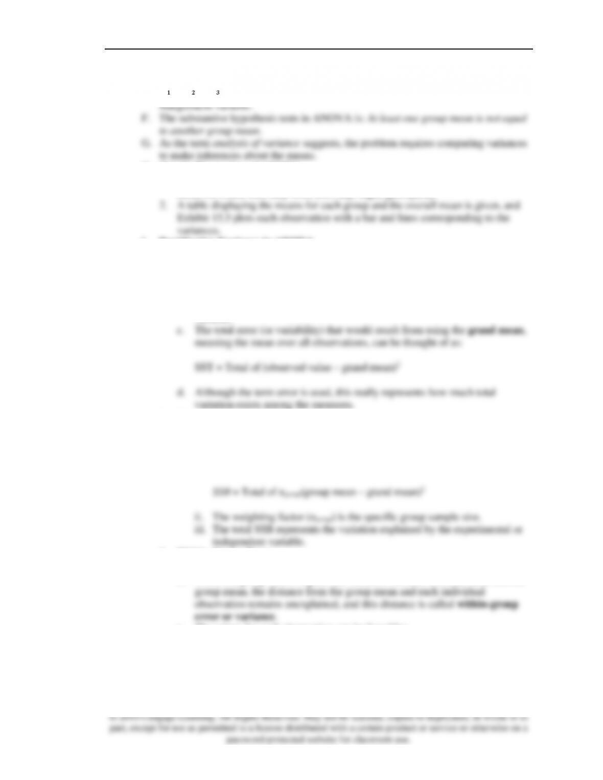
1. Data are given describing how much coffee respondents report drinking each day
based on which shift they work (i.e., day, night, graveyard).
I. Partitioning Variance in ANOVA
1. Total Variability
a. An implicit question with the use of ANOVA is “How can the dependent
variable best be predicted?”
b. Absent any additional information, the error in predicting an observation is
minimized by choosing the central tendency, or mean, for an interval
variable.
2. Between-Groups Variance
a. ANOVA tests whether “grouping” observations explains variance in the
dependent variable.
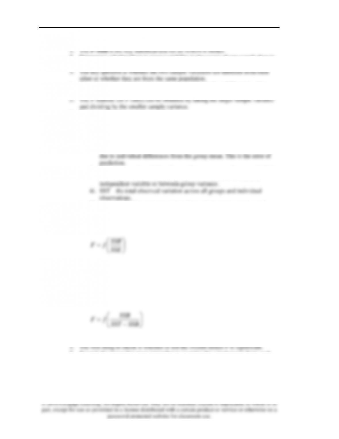
i. The between groups variance can be found by taking the total sum of
the weighted difference between group means and the overall mean:
3. Within-Group Error
a. Finally, error within each group would remain.
b. While the group means explain the variation between the total mean and the
c. The values for each observation can be found by:
SSE = total of (observed mean – group mean)2
d. The term total error variance is sometimes used to refer to SSE since it is
variability not accounted for by the group means.
=
=
Chapter Fifteen: Testing for Differences Between Groups and for Predictive Relationships 416
J. The F-Test
2. Determines whether there is more variability in the scores of one sample than in
the scores of another sample.
4. Thus, the test breaks down the variance in a total sample and illustrates why
ANOVA is analysis of variance.
6. Degrees of freedom must be specified.
7. Using Variance Components to Compute F-Ratios
a. In ANOVA, the basic consideration for the F-test is identifying the relative
size of variance components.
b. The three forms of variation described briefly are:
i. SSE—variation of scores due to random error or within-group variation
ii. SSB—systematic variation of scores between groups due to manipulation
of an experimental variable or group classifications of a measured
c. Thus, total variability can be partitioned into within-group variance and
between-group variance.
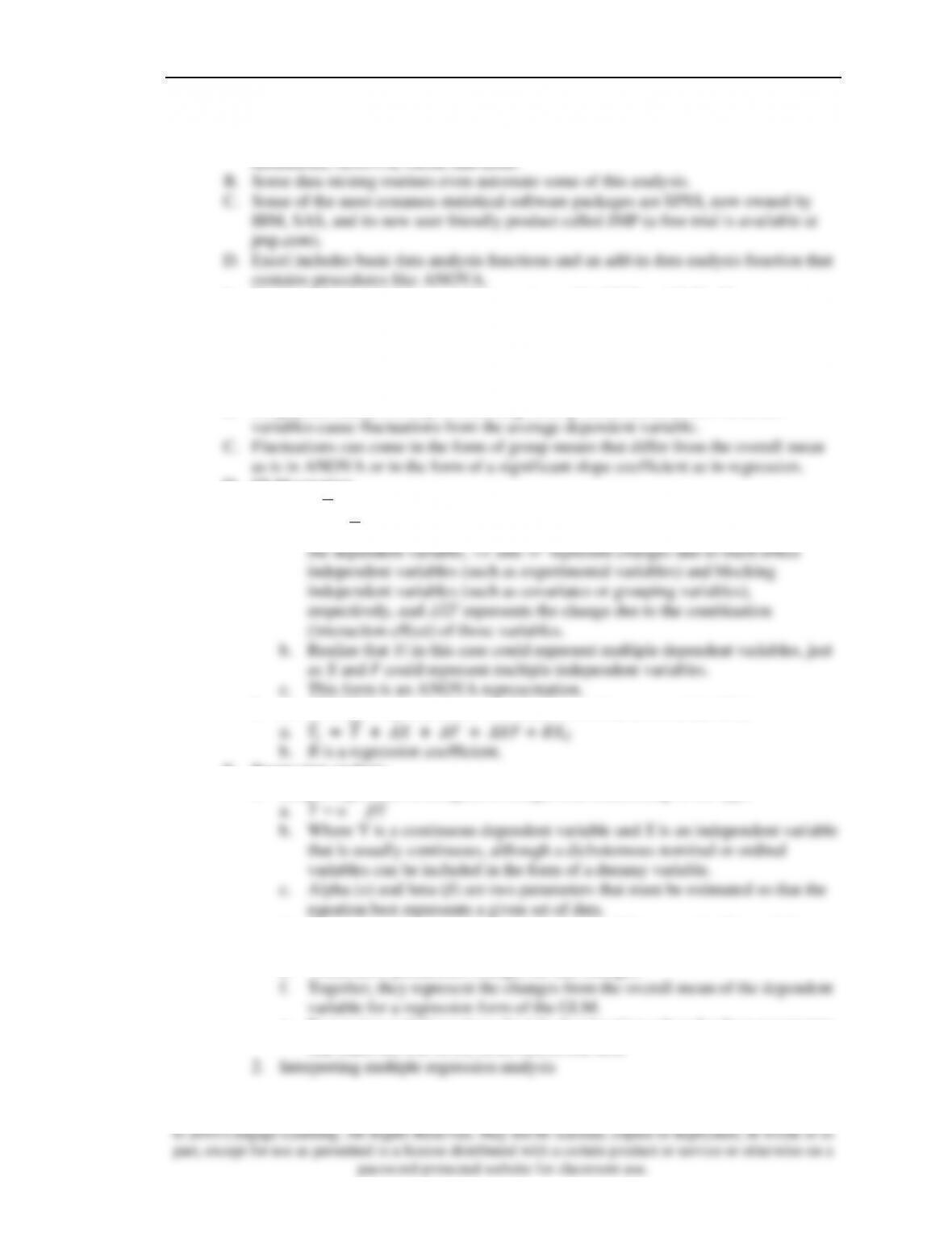
d. The F-distribution is a function of the ratio of these two sources of variance:
=SSE
SSB
fF
e. A larger ratio of variance between groups to variance within groups implies a
greater value of F.
f. If the F-value is large, the results are likely to be statistically significant.
8. A Different but Equivalent Representation
a. F also can be thoughts of as a function of the between group variance and
total variance.
−
K. Practically Speaking
2. Second, the researcher must remember to examine the actual means from each
group to properly interpret the result.
VI. STATISTICAL SOFTWARE
Chapter Fifteen: Testing for Differences Between Groups and for Predictive Relationships 417
A. The marketing research analyst has access to statistical software that facilitates
statistical analysis by quickly and easily providing results for t-tests, cross-
tabulations, ANOVA, GLM, and more.
E. However, for marketing researchers, packages like SPSS and JMP offer an easy to
use interface and a standardized approach to statistics.
VII. GENERAL LINEAR MODEL
A. Multivariate dependence techniques are variants of the general linear model (GLM).
B. Simply, the GLM is a way of modeling some process based on how different
D. GLM equation
1. 𝑌
𝑖 = 𝑌 + 𝛥𝑋 + 𝛥𝐹 + 𝛥𝑋𝐹
a. Here, 𝑌 represents a constant, which can be thought of as the overall mean of
2. An ANCOVA representation would add a continuous covariate (Xc):
E. Regression analysis
1. Simple regression investigates a straight-line relationship of the type:
d. These two parameters determine the height of the regression line and the
angle of the line relative to horizontal.
e. When these parameters change, the line changes.
g. Regression techniques have the job of estimating values for these parameters
that make the line fit the observations the best.
Chapter Fifteen: Testing for Differences Between Groups and for Predictive Relationships 418
a. Multiple regression analysis is an extension of simple regression analysis
3. Parameter estimate choices
d. A Y–intercept term is sometimes referred to as a constant because α
represents a fixed point.
e. An estimated slope coefficient is sometimes referred to as a regression
weight, regression coefficient, parameter estimate, or sometimes even as a
path estimate.
g. Researchers often explain regression results by referring to a standardized
regression coefficient (β).
i. A standardized regression coefficient, like a correlation coefficient,
provides a common metric allowing regression results to be compared to
h. Researchers use shorthand to label regression coefficients as either “raw” or
“standardized.”
j. The bottom line is that when the actual units of measurement are the focus of
analysis, such as might be the case in trying to forecast sales during some
period, raw (unstandardized) coefficients are most appropriate.
4. Steps in interpreting a multiple regression model
a. Examine the model F-test. If the test result is not significant, the model
should be dismissed and there is no need to proceed to further steps.
Chapter Fifteen: Testing for Differences Between Groups and for Predictive Relationships 419
© 2016 Cengage Learning. All Rights Reserved. May not be scanned, copied or duplicated, in whole or in
part, except for use as permitted in a license distributed with a certain product or service or otherwise on a
password-protected website for classroom use.
c. Examine the model 𝑅2. No cutoff values exist that can distinguish an
acceptable amount of explained variation across all regression models.
However, the absolute value of 𝑅2 is more important when the researcher is
more interested in prediction than explanation. In other words, the regression
is run for pure forecasting purposes. When the model is more oriented toward
explaining which variables are most important in explaining the dependent
variable, cutoff values for the model 𝑅2 are inappropriate.
Inflation Factors (VIF). Most statistical packages allow these to be
computed. VIFs of between 1 and 2 are generally not indicative of problems
with multicollinearity. As they become larger, the results become more
susceptible to interpretation problems because of overlap in the independent
variables.
QUESTIONS FOR REVIEW AND CRITICAL THINKING/ANSWERS
1. What tests of difference are appropriate in the following situations?
a. Average campaign contributions (in $) of Democrats, Republicans, and independents are
to be compared.
b. Advertising managers and brand managers respond “yes,” “no,” or “not sure” to an
attitude question. The advertising and brand managers’ responses are to be compared.
c. One-half of a sample received an incentive in a mail survey while the other half did not.
A comparison of response rates is desired.
d. A researcher believes coupon links pushed through Facebook.com will generate more
sales than coupon links pushed through Twitter.com
e. A manager wishes to compare the job performance of a salesperson before ethics training
with the performance of that same salesperson after ethics training.
Chapter Fifteen: Testing for Differences Between Groups and for Predictive Relationships 420
© 2016 Cengage Learning. All Rights Reserved. May not be scanned, copied or duplicated, in whole or in
part, except for use as permitted in a license distributed with a certain product or service or otherwise on a
password-protected website for classroom use.
In this case, the same respondent is measured twice – performance before and after ethics
training. A paired samples t-test is appropriate in this situation.
2. Perform a 2 test on the following data (hint: set up a spreadsheet to perform the calculations
as a good way of learning what the test really does):
a. Managers and line employees differ in their response to: “Increased regulation is the best
way to ensure safe products.”
Agree
Disagree
No Opinion
Managers
58
66
8
Line Employees
34
24
10
Totals
92
90
18
b. Test the following hypotheses with the data below; Hb: Women are more likely to have a
pinterest.com account. Do you have a pinterest.com account?
Yes
No
Male
25
75
Female
80
20
The 2 = 2.66 and is significant.
3. Interpret the following computer cross-tab output including a 2 test. Variable EDUCATION
is a response to “What is your highest level of educational achievement?” HS means a high
school diploma, SC means some college, BS means a bachelor’s degree, and MBA means a
master of business administration. Variable WIN is how well the respondent did on a set of
casino games of chance. A 1 means they would have lost more than $100, a 2 means they
approximately broke even, and a 3 means they won more that $100. What is the result of
exploring a research question that education influences performance on casino gambling?
Comment on your conclusion and any issues in interpreting the result. (Note: See SAS output
in textbook.)