© 2016 Cengage Learning. All Rights Reserved. May not be scanned, copied or duplicated, in whole or in
part, except for use as permitted in a license distributed with a certain product or service or otherwise on a
password-protected website for classroom use.
4.00 12 . 0000
.00 13 .
12.00 16 . 000000000000
.00 17 .
6.00 Extremes (>=20.0)
Stem width: 1
Each leaf: 1 case(s)
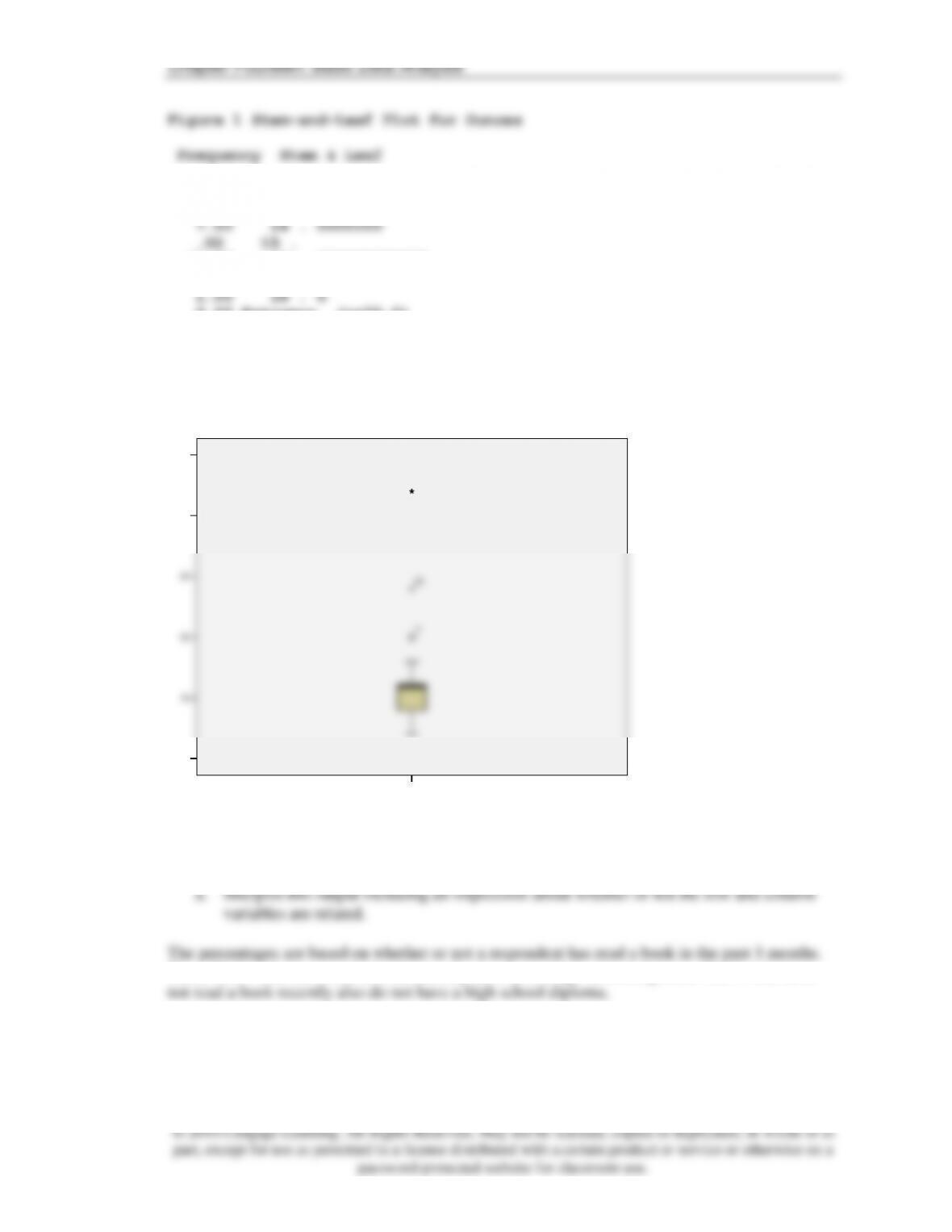
Figure 2. Box and Whiskers Plot
7. The following computer output (see textbook) shows a cross-tabulation of frequencies and
provides frequency number (N) and row (R) percentages.
Thus, 73.8% who have read a book recently also have a high school diploma. 55.6% who have
ounces
35
30
25
20
15
10
3
14
23
© 2016 Cengage Learning. All Rights Reserved. May not be scanned, copied or duplicated, in whole or in
part, except for use as permitted in a license distributed with a certain product or service or otherwise on a
password-protected website for classroom use.
8. List and describe at least three basic data transformations.
Data transformation is the process of changing the data from their original form to a format
9. What conditions suggest that a ratio variable should be transformed into a dichotomous (two
group) variable represented with dummy coding?
10. [Ethics Question] A data processing analysis for a research supplier finds that preliminary
computer runs of survey results show that consumers love a client’s new product. The
employee buys a large block of the client’s stock. Is this ethical?
11. [Internet Question] Use a Web site such as http://www.styledrops.com to find some prices for
4 Prada handbags, 4 Gucci handbags, 4 Yves Saint Laurent handbags, 4 Burberry handbags,
and 4 Ferragamo handbags. Enter these into a spreadsheet. Using the lowest priced Prada
handbag as a base, compute an index displaying the price of all other handbags. Which brand
offers the best value in your opinion? Compute the appropriate statistic for central tendency
using a spreadsheet or some other software. Use the chart feature (in Excel or another
package) to depict the prices as a frequency distribution.
© 2016 Cengage Learning. All Rights Reserved. May not be scanned, copied or duplicated, in whole or in
part, except for use as permitted in a license distributed with a certain product or service or otherwise on a
password-protected website for classroom use.
12. Describe the basic hypothesis testing procedure.
The process can be described as follows:
2. A sample is obtained and the relevant variables are measured.
3. The measured value obtained in the sample is compared to the value either stated
13. What is a p-value and how is it used?
0.05, or 0.01). If the p-value, which stands for probability-level and is essentially another name
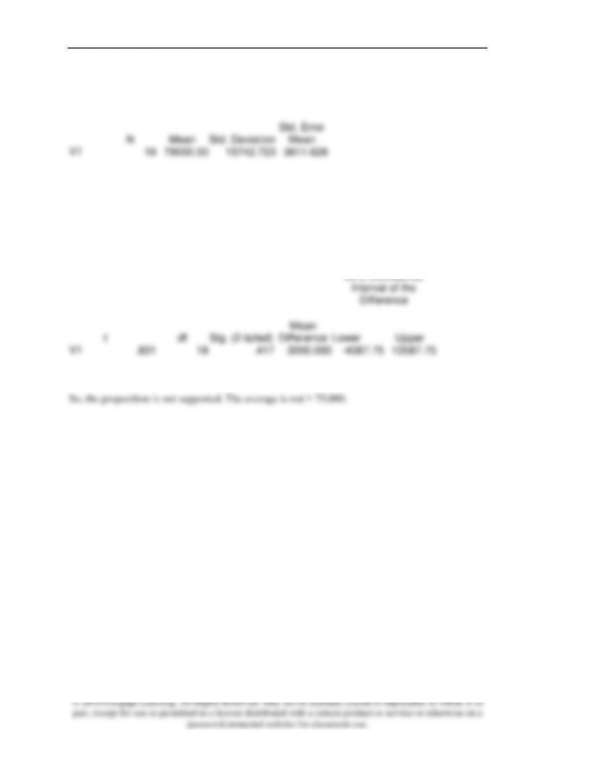
14. A researcher is asked to determine whether or not a productivity objective (in dollars) of
better than $75,000 per employee is possible. A productivity test is done involving 20
employees. What conclusion would you reach? The sales results are as follows:
Chapter Fourteen: Basic Data Analysis
One-Sample Statistics
N
Mean
Std. Deviation
Std. Error
Mean
V1
19
78000.00
15742.723
3611.628
One-Sample Test
Test Value = 75000
t
df
Sig. (2-tailed)
Mean
Difference
95% Confidence
Interval of the
Difference
Lower
Upper
V1
.831
18
.417
3000.000
-4587.75
10587.75
Chapter Fourteen: Basic Data Analysis
RESEARCH ACTIVITIES
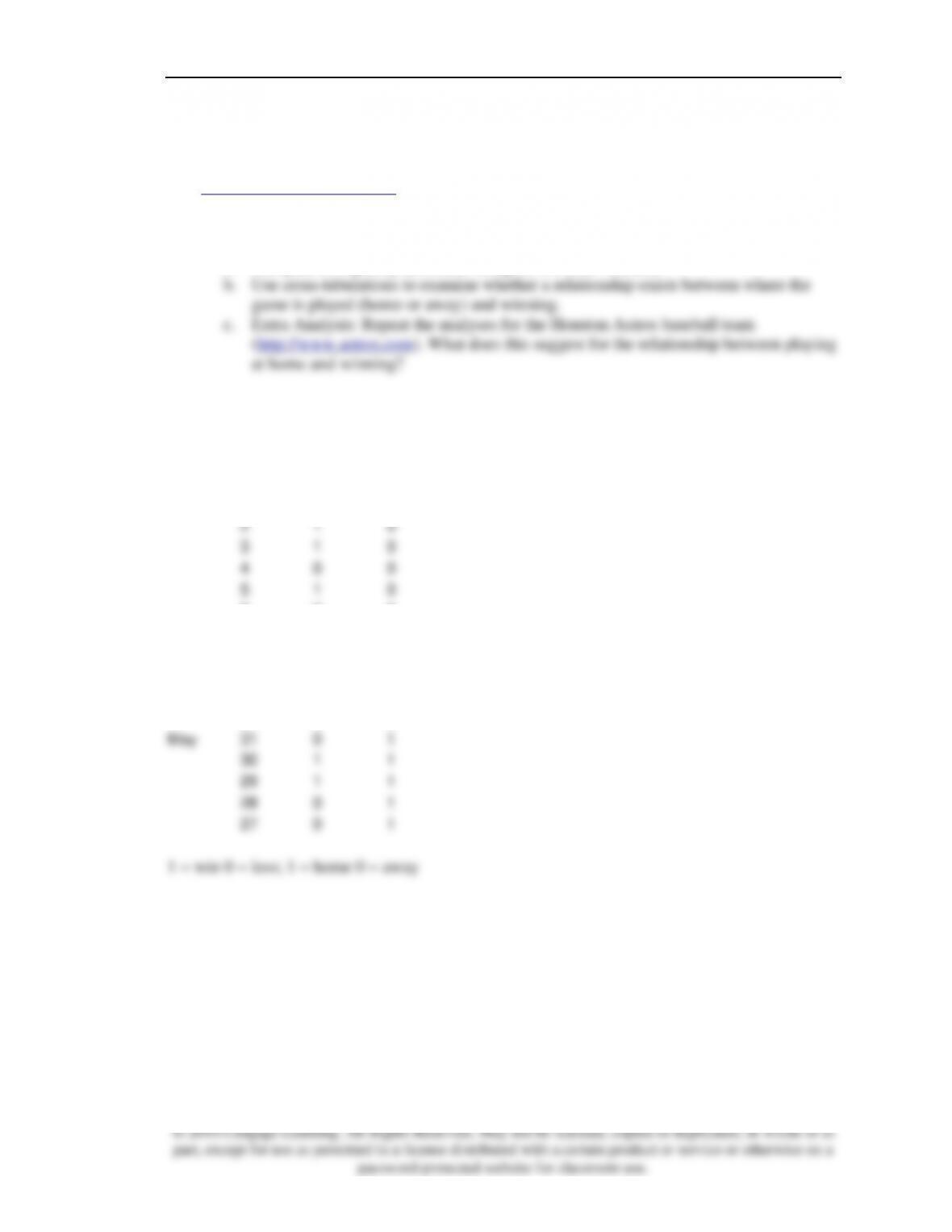
1. [Internet Question] Go to the web site for the Chicago Cubs baseball team
(http://chicago.cubs.mlb.com). Use either the schedule listing or the stats information to find
their record in the most recent season. Create a data file with a variable indicating whether
each game was won or lost and a variable indicating whether the game was played at home in
Wrigley Field or away from home. Using computerized software like SPSS or SAS,
a. Compute a frequency table and histogram for each variable.
Answers will vary depending on the year from which the data are taken. The student has to create
a data set like this which can easily be obtained from the web site. This data is from a few games
in the 2006 season:
day
win/loss
home/away
June
1
1
0
2
1
0
3
1
0
4
0
0
5
1
0
6
0
0
7
0
0
8
0
0
9
1
0
10
1
0
11
1
0
May
31
0
1
30
1
1
29
1
1
28
0
1
27
0
1
Then, this can be put in SPSS or SAS to get the analysis requested. While students’ results will be
different depending on when this exercise is performed, they will look something like this:
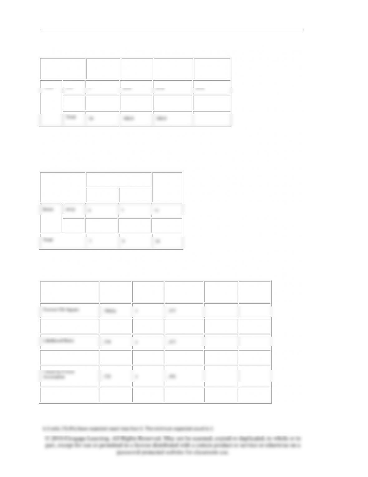
Chapter Fourteen: Basic Data Analysis
win
Frequency
Percent
Valid Percent
Cumulative
Percent
Valid
loss
7
43.8
43.8
43.8
win
9
56.3
56.3
100.0
Total
16
100.0
100.0
home * win Crosstabulation
Count
win
Total
loss
win
home
away
4
7
11
home
3
2
5
Total
7
9
16
Chi-Square Tests
Value
df
Asymp. Sig. (2-
sided)
Exact Sig. (2–
sided)
Exact Sig. (1–
sided)
Pearson Chi-Square
.780(b)
1
.377
Continuity Correction(a)
.115
1
.734
Likelihood Ratio
.779
1
.377
Fisher’s Exact Test
.596
.365
Linear-by-Linear
Association
.732
1
.392
N of Valid Cases
16
a Computed only for a 2×2 table
Chapter Fourteen: Basic Data Analysis
Questions
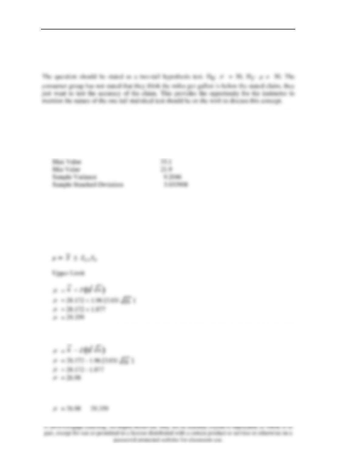
1. Formulate a statistical hypothesis appropriate for the consumer group’s purpose.
2. Calculate the mean average miles per gallon. Compute the sample variance and sample
standard deviation.
Mean 28.172
Median 28.7
Mode 30.9
3. Construct the appropriate statistical test for your hypothesis, using a 0.05 significance level.
H0: = 30
H1: 30
Using a hand calculation the results are as follows:
Lower Limit
Thus, the confidence interval for the hypothesis test would be:
Chapter Fourteen: Basic Data Analysis
© 2016 Cengage Learning. All Rights Reserved. May not be scanned, copied or duplicated, in whole or in
part, except for use as permitted in a license distributed with a certain product or service or otherwise on a
password-protected website for classroom use.
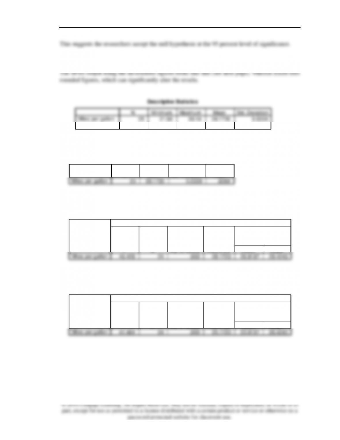
This suggests the researchers accept the null hypothesis at the 95 percent level of significance.
4. Use at least two different software packages to conduct the statistical test. For instance, use
Excel and use a statistics package like SPSS or JMP. Are the results the same? Comment.
Descriptive Statistics
25
21.90
35.10
28.1720
3.0339
25
Miles per gallon
Valid N (lis twis e)
N
Minimum
Maximum
Mean
Std. Deviation
One–Sample Statistics
25
28.1720
3.0339
.6068
Miles per gallon
N
Mean
Std. Deviation
Std. Error
Mean
One-Sample Test
46.429
24
.000
28.1720
26.9197
29.4243
Miles per gallon
t
df
Sig. (2-tailed)
Mean
Difference
Lower
Upper
95% Confidence
Interval of the
Difference
Test Value = 0
One-Sample Test
41.484
24
.000
25.1720
23.9197
26.4243
Miles per gallon
t
df
Sig. (2-tailed)
Mean
Difference
Lower
Upper
95% Confidence
Interval of the
Difference
Test Value = 3.0