
Chapter Thirteen: Big Data Basics: Describing Samples and Populations
Chapter 13
Big Data Basics: Describing
Samples and Populations
AT-A-GLANCE
I. Introduction
II. Descriptive Statistics and Basic Inferences
A. What are sample statistics and population parameters?
1. Frequency distributions
3. Top-box/bottom-box scores
B. Central tendency metrics
2. The median
3. The mode
C. Dispersion metrics
1. The range
3. Why use the standard deviation?
a. Variance
b. Standard deviation
III. Distinguish among Population, Sample and Sample Distribution
IV. Central-Limit Theorem
V. Estimation of Parameters and Confidence Intervals
A. Point estimates
B. Confidence intervals
VI. Sample Size
A. Random error and sample size
B. Factors in determining sample size for questions involving means
C. Estimating sample size for questions involving means
VII. Assess the potential for nonresponse bias
Chapter Thirteen: Big Data Basics: Describing Samples and Populations
LEARNING OUTCOMES
1. Use basic descriptive statistics to analyze data and make basic inferences about population
metrics.
3. Explain the central-limit theorem.
5. Understand major issues in specifying sample size.
CHAPTER VIGNETTE: It’s a Numbers Game
Marketing depends a great deal on numbers and on mathematics – particularly statistics. Never
has this been more true than in the big data era, where companies are seeking marketing
researchers capable of analyzing all the numbers that are stored about customers and their
choices. The key to using all of these numbers, which essentially comprise raw data, is to
SURVEY THIS!
Students are asked to imagine that a marketing manager is trying to determine how many students
have only one e-mail account that they use regularly, and then to answer the following questions:
1. What is the proportion of students in the sample that have more than one e-mail account?
2. If the student population is 5 million students, what sample size is needed to estimate the
actual proportion of students with more than one active e-mail account within ±1
percent?
3. What sample size is needed to estimate the actual proportion of students with more than
one active e-mail account within ±5 percent?
4. If the decision to launch this marketing activity involves an investment of approximately
$75,000 for this company (with median annual revenues of $3M), what level of precision
would you recommend?
Chapter Thirteen: Big Data Basics: Describing Samples and Populations
RESEARCH SNAPSHOTS
➢ Are You Facebook Normal?
Are you normal? A quiz at www.blogthings.com may give you an answer to that question (a
site that offers many quizzes where one can compare themselves with others and find things
out about themselves – like what is your number? Or color?) It consists of 20 questions
covering things like whether or not you change towels every day, whether you have closer to
$40 or $100 on hand, whether you are comfortable using the bathroom with another person in
➢ Target and Wal-Mart Shoppers Really Are Different
Scarborough Research sampled over 220,000 adults to compare consumers who shop
exclusively at either Target or Wal-Mart. The largest share (40 percent) named both stores
when asked to identify the stores at which they had shopped during the preceding three
months. However, 31 percent shopped at Wal-Mart but not Target, and 12 percent shopped at
TIPS OF THE TRADE
➢ Measures of central tendency provide overall summaries of the level to which some
phenomenon exists on average. The appropriate central tendency statistic varies with the
nature of the data.
▪ The mean is the most commonly used measure of central tendency.
➢ Sample size estimates often require some estimate of the standard deviation that will exist in
the sample.
▪ Larger samples allow predictions with greater precision that can be expressed over a
smaller range.
Chapter Thirteen: Big Data Basics: Describing Samples and Populations
➢ Low response rates (under 10 percent) are common in marketing research.
OUTLINE
I. INTRODUCTION
A. All the statistics in this chapter are univariate in the sense that only one variable is
II. DESCRIPTIVE STATISTICS AND BASIC INFERENCES
A. Raw data are just numbers with words and little meaning
1. The most basic statistical tools for summarizing information from data include
2. Statistics like these often provide a summary number that allows analysts to
4. The combination of summary metrics from basic statistics and a valid sample
proves vital in making effective marketing and business decisions.
6. Two applications of statistics exist:
a. To describe characteristics of the population or sample and
b. To generalize from a sample to a population.
B. What are Sample Statistics and Population Parameters?
1. The primary purpose of inferential statistics is to make a judgment about the
population, or the collection of all elements about which one seeks information.
3. Sample statistics are measures computed from sample data.
5. We will generally use Greek lowercase letters to denote population parameters
(e.g.,
or
) and English letters to denote sample statistics (e.g., X or S).
6. Frequency Distributions
a. Constructing a frequency table or frequency distribution is one of the most
common means of summarizing a set of data.
© 2016 Cengage Learning. All Rights Reserved. May not be scanned, copied or duplicated, in whole or in
part, except for use as permitted in a license distributed with a certain product or service or otherwise on a
password-protected website for classroom use.
100.
d. Probability is the long-run relative frequency with which an event will
7. Proportions
8. Top-Box/Bottom-Box Scores
a. A top box score generally refers to the portion of respondents who choose
the most favorable response toward a company.
b. Typically, this means the portion that would highly recommend a business to
C. Central Tendency Metrics
2. The Mean
a. The mean is simply the arithmetic average, and it is a common measure of
central tendency.
3. The Median
a. The median is the midpoint of the distribution, or the 50th percentile.
4. The Mode
a. The mode is the measure of central tendency that merely identifies the value
that occurs most often.
D. Dispersion Metrics
Chapter Thirteen: Big Data Basics: Describing Samples and Populations
(a) The variance does have one major drawback—it reflects a unit of
measurement that has been squared.
(b) Because of this, statisticians have taken the square root of the
variance.
(c) The square root of the variance for distribution is called the
standard deviation.
(d) S is the symbol for the sample standard deviation, while is the
symbol for the population standard deviation.
III. DISTINGUISH BETWEEN POPULATATION, SAMPLE AND SAMPLE
DISTRIBUTION
A. The Normal Distribution
1. One of the most common probability distributions in statistics is the normal
distribution (a.k.a., the normal curve).
3. The standardized normal distribution is a specific normal curve that has
several characteristics
1.0.
4. The standardized normal distribution is a purely theoretical probability
distribution, but it is the most useful distribution in inferential statistics.
5. The standardized normal distribution is extremely valuable because we can
translate or transform any normal variable, X, into the standardized value, Z.
6. Computing the standardized value, Z, of any measurement expressed in original
units is simple:
a. Subtract the mean from the value to be transformed, and divide by the
standard deviation (all expressed in original units).
b. In the formula note that σ, the population standard deviation, is
Chapter Thirteen: Big Data Basics: Describing Samples and Populations
𝑍 = 7,500−9,000
500 = −3.00
𝑍 = 9,625−9,000
500 = 1.25
When Z = 3.00, the area under the curve (probability) equals .499
When Z = 1.25, the area under the curve (probability) equals .394
Thus, the total area under the curve is .499 + .394 = .893
The area under the curve portraying this computation is the shaded
area in Exhibit 17.12. Thus, the sales manager knows there is a .893
probability that sales will be between 7,500 and 9,625.
B. Population Distribution and Sample Distribution
1. Three additional types of distribution must be defined:
a. Population distribution
b. Sample distribution
c. Sampling distribution
2. A frequency distribution of the population elements is called a population
distribution.
3. The population distribution has its mean and standard deviation represented by
the Greek letters µ and σ.
5. The sample mean is designated with 𝑋, and the sample standard deviation is
designated S.
6. Sampling Distribution
a. However, we must now introduce another distribution: the sampling
distribution of the sample mean.
b. A sampling distribution is a theoretical probability that shows the
c. The sampling distribution’s mean is called the expected value of the statistic.
d. The expected value of the mean of the sampling distribution is equal to µ.
IV. CENTRAL-LIMIT THEOREM
A. The central-limit theorem states: As the sample size, n, increases, the distribution of
√𝑛 ).
B. The central-limit theorem works regardless of the shape of the original population
distribution.
C. This theoretical knowledge about distributions can be used to solve two very
practical marketing research problems:
© 2016 Cengage Learning. All Rights Reserved. May not be scanned, copied or duplicated, in whole or in
part, except for use as permitted in a license distributed with a certain product or service or otherwise on a
password-protected website for classroom use.
11. There will be a random sampling error, which is the difference between the
survey results and the results of surveying the entire population.
VI. SAMPLE SIZE
A. Random Error and Sample Size
1. Random sampling error varies with samples of different sizes.
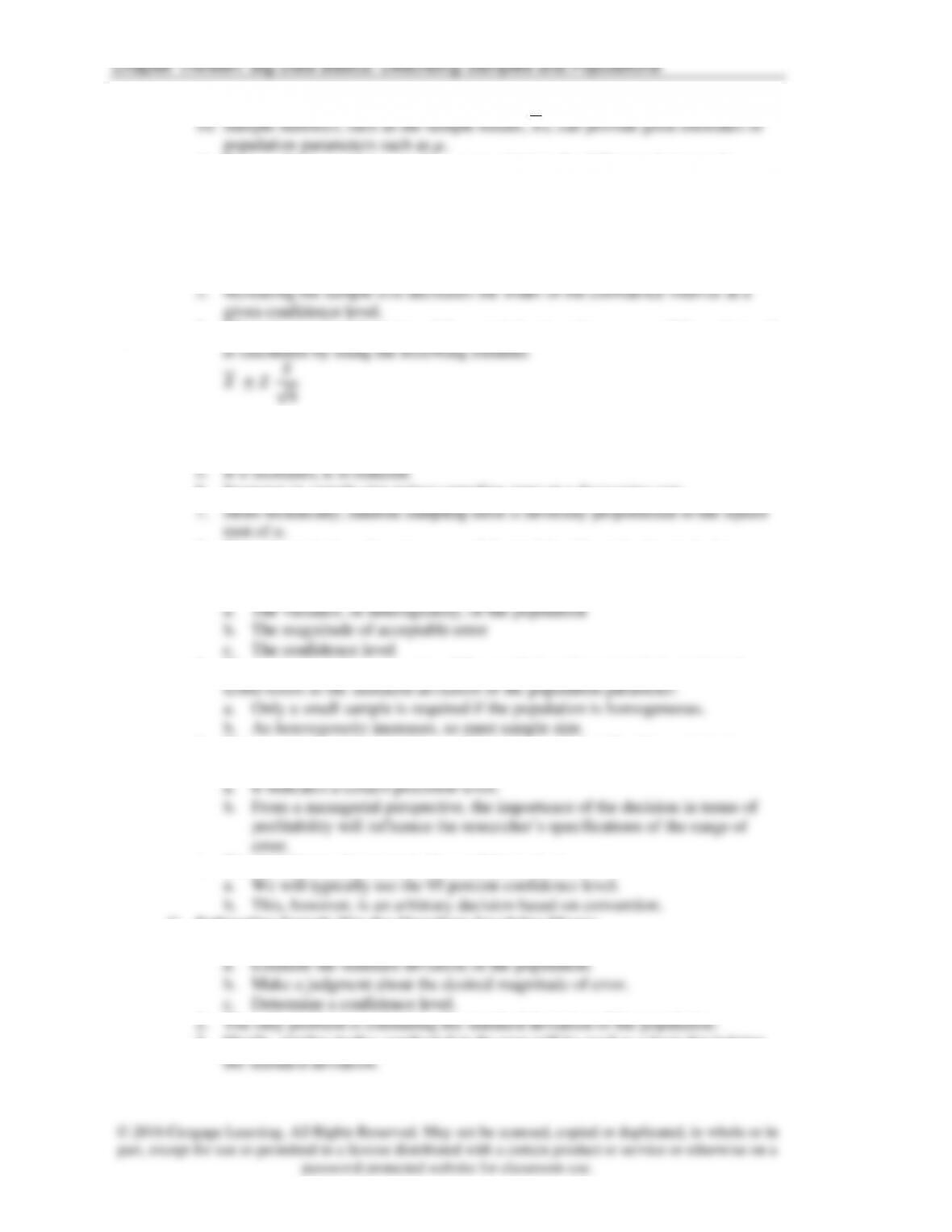
3. When the standard deviation of the population is unknown, a confidence interval
4. Observe that the equation for the plus or minus error factor in the confidence
interval includes n, the sample size.
6. Increases in sample size reduce sampling error at a decreasing rate.
8. Thus, the main issue becomes ones of determining the optimal sample size.
B. Factors in Determining Sample Size for Questions Involving Means
1. Three factors are required to specify sample size:
2. The variance, or heterogeneity, of the population characteristic in statistical
3. The magnitude of error, or the confidence interval, is defined in statistical terms
as E, and indicates how precise the estimate must be.
4. The third factor of concern is the confidence level.
C. Estimating Sample Size for Questions Involving Means
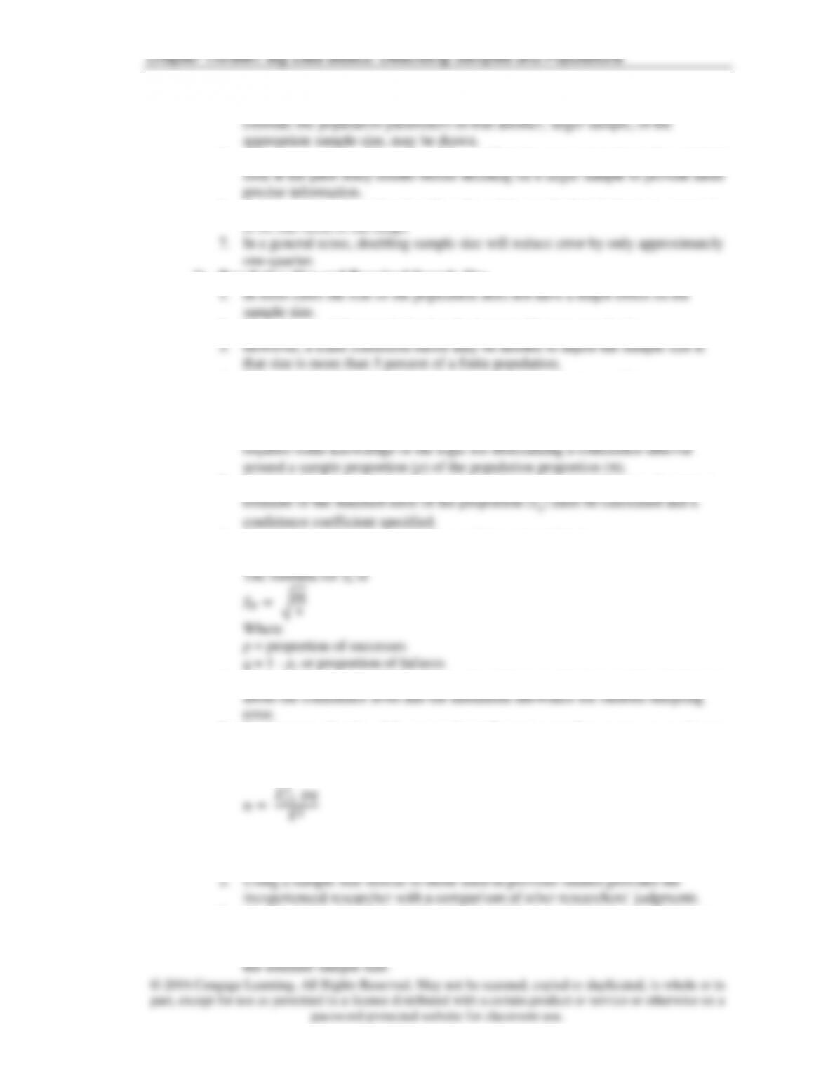
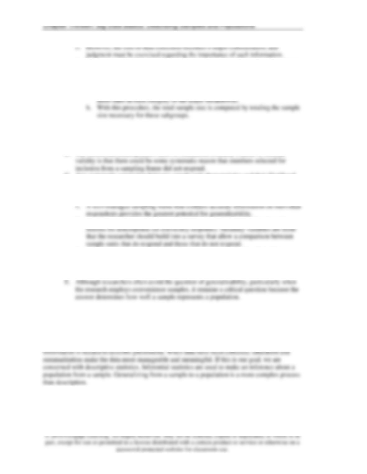
1. The researcher must follow three steps:
3. Ideally, similar studies conducted in the past will be used as a basis for judging
© 2016 Cengage Learning. All Rights Reserved. May not be scanned, copied or duplicated, in whole or in
part, except for use as permitted in a license distributed with a certain product or service or otherwise on a
password-protected website for classroom use.
6. Another consideration stems from most researchers’ need to analyze the various
subgroups within the sample.
7. There is a judgmental rule of thumb for selecting minimum subgroup sample
size:
a. Each subgroup to be separately analyzed should have a minimum of 100 or
VII. ASSESS THE POTENTIAL FOR NONRESPONSE BIAS
A. Nonresponse bias, in particular the bias caused when sample units provide no
response, can significantly damage generalizability.
B. The reason that nonresponders must be considered routinely a threat to external
C. Any systematic connection between sample unit characteristics and their likelihood
to respond is a potential source for bias.
D. Some basic procedures can be followed in an effort to increase confidence in the
generalizability of the sample:
2. Auxiliary variables provide a useful means of detecting potential systematic
3. A high response rate in and of itself does not guarantee freedom from bias.
4. Post-hoc sampling procedures can be employed, which adjust the contact of
individuals in a way that tries to over-contact types of people that were not likely
to respond to the initial sampling plan.
QUESTIONS FOR REVIEW AND CRITICAL THINKING/ANSWERS
1. What is the difference between descriptive and inferential statistics?