
1
Chapter 12 – Examining Relationships in Quantitative Research
Chapter 12
Examining Relationships in Quantitative
Research
Learning Objectives (PPT slides 12-2 and 12–3)
1. Understand and evaluate the types of relationships between variables.
2. Explain the concepts of association and co-variation.
3. Discuss the differences between Pearson correlation and Spearman correlation.
Key Terms and Concepts
1. Beta coefficient
2. Bivariate regression analysis
3. Coefficient of determination (r2)
4. Covariation
5. Curvilinear relationship
6. Homoskedasticity
7. Heteroskedasticity
8. Least squares procedure

2
Chapter 12 – Examining Relationships in Quantitative Research
Chapter Summary by Learning Objectives
Understand and evaluate the types of relationships between variables.
Relationships between variables can be described in several ways, including presence, direction,
strength of association, and type. Presence tells us whether a consistent and systematic relationship
exists. Direction tells us whether the relationship is positive or negative. Strength of association
tells us whether we have a weak or strong relationship, and the type of relationship is usually
described as either linear or nonlinear.
Explain the concepts of association and covariation.
The terms covariation and association refer to the attempt to quantify the strength of the
relationship between two variables. Covariation is the amount of change in one variable of interest
that is consistently related to change in another variable under study. The degree of association is a
numerical measure of the strength of the relationship between two variables. Both these terms refer
to linear relationships.
Discuss the differences between Pearson correlation and Spearman correlation.
Explain the concept of statistical significance versus practical significance.
Because some of the procedures involved in determining the statistical significance of a statistical
test include consideration of the sample size, it is possible to have a very low degree of association
between two variables show up as statistically significant (i.e., the population parameter is not
equal to zero). However, by considering the absolute strength of the relationship in addition to its
statistical significance, the researcher is better able to draw the appropriate conclusion about the
data and the population from which they were selected.

3
Chapter 12 – Examining Relationships in Quantitative Research
Understand when and how to use regression analysis.
Regression analysis is useful in answering questions about the strength of a linear relationship
between a dependent variable and one or more independent variables. The results of a regression
analysis indicate the amount of change in the dependent variable that is associated with a one-unit
Understand the value and application of structural modeling.
Structural modeling enables researchers to analyze complex multivariate models. The most
appropriate structural modeling method for marketing research applications is partial least squares
structural equation modeling (PLS-SEM). The PLS-SEM method is an extension of ordinary least
Chapter Outline
Opening Vignette: Data Mining Helps Rebuild Procter & Gamble as a Global Powerhouse
The opening vignette in this chapter describes how Procter & Gamble (P&G), a global player in
consumer household products, used information technology and customer relationship
management to design their brand building strategy. From internal employee surveys they
I. Examining Relationships between Variables (PPT slide 12-4)
Relationships between variables can be described in several ways, including presence, direction,
strength of association, and type (PPT slides 12-4 to 12-6). If a systematic relationship exists
4
Chapter 12 – Examining Relationships in Quantitative Research
An understanding of the strength of association also is important. Researchers generally categorize
the strength of association as no relationship, weak relationship, moderate relationship, or strong
relationship. If a consistent and systematic relationship is not present, then there is no relationship.
A weak association means the variables may have some variance in common, but not much. A
moderate or strong association means there is a consistent and systematic relationship, and the
relationship is much more evident when it is strong. The strength of association is determined by
the size of the correlation coefficient, with larger coefficients indicating a stronger association.
A linear relationship is much simpler to work with than a curvilinear relationship. If the
researchers know the value of variable X, then they can apply the formula for a straight line (Y = a
+ bX) to determine the value of Y. But when two variables have a curvilinear relationship, the
formula that best describes the linkage is more complex. Therefore, most marketing researchers
work with relationships they believe are linear.
Marketers are often interested in describing the relationship between variables they think influence
purchases of their product(s). There are four questions to ask about a possible relationship between
two variables.
• “Is there a relationship between the two variables of interest?”
• If there is a relationship, “How strong is that relationship?”
II. Covariation and Variable Relationships (PPT slide 12-5)
Covariation is the amount of change in one variable that is consistently related to the change in
another variable of interest (PPT slide 12-5). Another way of stating the concept of covariation is
that it is the degree of association between two variables. If two variables are found to change
together on a reliable or consistent basis, then we can use that information to make predictions that
will improve decision making about advertising and marketing strategies.
5
Chapter 12 – Examining Relationships in Quantitative Research
One way of visually describing the covariation between two variables is with the use of a scatter
diagram (PPT slide 12-5). A scatter diagram plots the relative position of two variables using
horizontal and vertical axes to represent the variable values. Exhibits 12.1 through 12.4 show some
examples of possible relationships between two variables that might show up on a scatter diagram.
• Exhibit 12.1 suggests there is no systematic relationship between X and Y and that there is
very little or no covariation shared by the two variables. The amount of covariation shared
by these two variables would be very close to zero.
• In Exhibit 12.2 the relationship between the two variables could be described as positive
because increases in the value of Y are associated with increases in the value of X. That is, if
researchers know the relationship between Y and X is a linear, positive relationship, they
would know the values of Y and X change in the same direction.
III. Correlation Analysis (PPT slide 12-6)
Scatter diagrams are a visual way to describe the relationship between two variables and the
covariation they share. But even though a picture is worth a thousand words, it is often more
convenient to use a quantitative measure of the covariation between two items.
The Pearson correlation coefficient is a statistical measure of the strength of a linear relationship
between two metric variables (PPT slide 12-6). It varies between –1.00 and 1.00, with 0
representing absolutely no association between two variables, and –1.00 or 1.00 representing a
perfect link between two variables. The correlation coefficient can be either positive or negative,
depending on the direction of the relationship between two variables. But the larger the correlation
coefficient, the stronger the association between two variables.
6
Chapter 12 – Examining Relationships in Quantitative Research
association between two variables. Some rules of thumb for characterizing the strength of the
association between two variables based on the size of the correlation coefficient are suggested in
Exhibit 12.5 (PPT slide 12-7).
A. Pearson Correlation Coefficient (PPT slide 12-8)
In calculating the Pearson correlation coefficient, researchers make several assumptions (PPT
slide 12-8). Following are their assumptions.
• First, researchers assume the two variables have been measured using interval- or
ratio-scaled measures.
B. SPSS Application—Pearson Correlation (PPT slide 12-9)
The text uses the restaurant database to examine the Pearson correlation. Exhibit 12.6 shows the
SPSS Pearson correlation (PPT slide 12-9).
C. Substantive Significance of the Correlation Coefficient (PPT slide 12-10)
When the correlation coefficient is strong and significant, the researchers can be confident that
the two variables are associated in a linear fashion. When the correlation coefficient is weak,
two possibilities must be considered.
• There is not a consistent, systematic relationship between the two variables.
• The association exists, but it is not linear, and other types of relationships must be
investigated further.
D. Influence of Measurement Scales on Correlation Analysis (PPT slide 12-11)
The Spearman rank order correlation coefficient is the recommended statistic to use when
7
Chapter 12 – Examining Relationships in Quantitative Research
two variables have been measured using ordinal scales (rank order) (PPT slide 12-11). If either
one of the variables is represented by rank order data, the best approach is to use the Spearman
rank order correlation coefficient, rather than the Pearson correlation.
E. SPSS Application—Spearman Rank Order Correlation (PPT slide 12-12)
This section takes students through the steps necessary to conduct the Spearman rank order
correlation using SPSS. The SPSS results for the Spearman correlation are shown in Exhibit
12.7 (PPT slide 12-12).
IV. What is Regression Analysis? (PPT slides 12-13 to 12-15)
Correlation can determine if a relationship exists between two variables. The correlation
coefficient also tells the researcher the overall strength of the association and direction of the
relationship between the variables. However, managers sometimes still need to know how to
describe the relationship between variables in greater detail. For example, a marketing manager
may want to predict future sales or how a price increase will affect the profits or market share of
the company. There are a number of ways to make such predictions.
• Extrapolation from past behavior of the variable
Extrapolation and guesses (educated or otherwise) usually assume that past conditions and
behaviors will continue into the future. They do not examine the influences behind the behavior of
interest. Consequently, when sales levels, profits, or other variables of interest to a manager differ
from those in the past, extrapolation and guessing do not explain why.
A couple of points should be made about the assumptions behind regression analysis.
• First, as with correlation, regression analysis assumes a linear relationship is a good
description of the relationship between two variables.
8
Chapter 12 – Examining Relationships in Quantitative Research
• Second, even though the terminology of regression analysis commonly uses the labels
dependent and independent for the variables, these labels do not mean we can say one
variable causes the behavior of the other.
• Regression analysis uses knowledge about the level and type of association between two
A. Fundamentals of Regression Analysis (PPT slides 12-16 to 12-19)
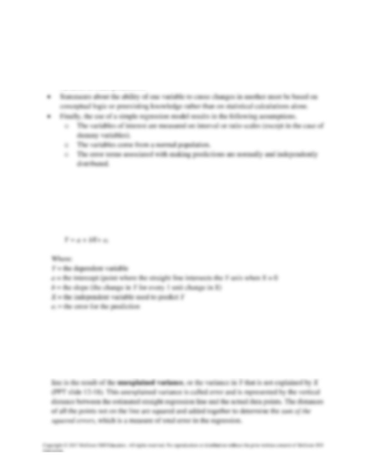
A fundamental basis of regression analysis is the assumption of a straight line relationship
between the independent and dependent variables. This relationship is illustrated in Exhibit
12.9 (PPT slide 12-16). The general formula for a straight line is:
In regression analysis, the researchers examine the relationship between the independent
variable X and the dependent variable Y. To do so, they use the actual values of X and Y in their
data set and the computed values of a and b. The calculations are based on the least squares
procedure (PPT slide 12-18). The least squares procedure determines the best-fitting line by
minimizing the vertical distances of all the data points from the line, as shown in Exhibit 12.10.
The best-fitting line is the regression line (PPT slide 12-19). Any point that does not fall on the

9
Chapter 12 – Examining Relationships in Quantitative Research
In the case of bivariate regression analysis, researchers look at one independent variable and
one dependent variable. However, managers frequently want to look at the combined influence
of several independent variables on one dependent variable. Multiple regression is the
appropriate technique to measure multivariate relationships.
B. Developing and Estimating the Regression Coefficients (PPT slides 12-20)
Regression uses an estimation procedure called ordinary least squares (OLS) that guarantees
the line it estimates will be the best fitting line. Ordinary least squares is a statistical
procedure that results in equation parameters (a and b) that produce predictions with the lowest
C. SPSS Application—Bivariate Regression (PPT slide 12-21)
This section illustrates bivariate regression analysis using the Santa Fe Grill database. Exhibit
12.11 contains the results of the bivariate regression analysis (PPT slide 12-21).
D. Significance (PPT slide 12-22)
Once the statistical significance of the regression coefficients is determined, the first question
about relationship is answered, “Is there a relationship between the dependent and independent
variable?” A second question to ask is “How strong is that relationship?” The output of
regression analysis includes the coefficient of determination, or r2—which describes the
amount of variation in the dependent variable associated with the variation in the independent

10
Chapter 12 – Examining Relationships in Quantitative Research
that the researcher’s dependent measure won’t change very much for a given unit change in the
independent measure.
E. Multiple Regression Analysis (PPT slide 12-23)
In most problems faced by managers, there are several independent variables that need to be
examined for their influence on a dependent variable. Multiple regression analysis is a
statistical technique which analyzes the linear relationship between a dependent variable and
multiple independent variables by estimating coefficients for the equation for a straight line
(PPT slide 12-23). Multiple independent variables are entered into the regression equation, and
for each variable a separate regression coefficient is calculated that describes its relationship
with the dependent variable.
With the addition of more than one independent variable, the researchers have some new issues
to consider. One is the possibility that each independent variable is measured using a different
scale. To solve this problem, the researchers calculate the standardized regression coefficient. It
is called a beta coefficient (PPT slide 12-23). It is an estimated regression coefficient that has
been recalculated to have a mean of 0 and a standard deviation of 1. Such a change enables
independent variables with different units of measurement to be directly compared on their
F. Statistical Significance (PPT slide 12-24)
After the regression coefficients have been estimated, the researcher must examine the
statistical significance of each coefficient. Each regression coefficient is divided by its standard
error to produce a t statistic, which is compared against the critical value to determine whether

11
Chapter 12 – Examining Relationships in Quantitative Research
does not change at all as the value of the statistically insignificant independent variable
changes.
When using multiple regression analysis, it is important to examine the overall statistical
significance of the regression model. The amount of variation in the dependent variable the
researchers have been able to explain with the independent measures is compared with the total
G. Substantive Significance (PPT slide 12-25)
Once the researchers have estimated the regression equation, they need to assess the strength of
the association. The multiple r2 or multiple coefficient of determination describes the strength
of the relationship between all the independent variables in our equation and the dependent
variable. The larger the r2 measure, the more of the behavior of the dependent measure is
associated with the independent measures the researchers are using to predict it.
To summarize, the elements of a multiple regression model to examine in determining its
significance include the following:
• r2
• model F statistic
The appropriate procedure to follow in evaluating the results of a regression analysis is given
below.
• Assess the statistical significance of the overall regression model using the F statistic and
its associated probability
H. Multiple Regression Assumptions (PPT slides 12-26 and 12-27)
The ordinary least squares approach to estimating a regression model requires that several

12
Chapter 12 – Examining Relationships in Quantitative Research
assumptions be met. The more important assumptions are given below.
• Linear relationship
The linearity assumption was illustrated in Exhibits 12.9 and 12.10. Exhibit 12.12 illustrates
heteroskedasticity—the pattern of covariation around the regression line is not constant
around the regression line, and varies in some way when the values change from small to
medium and large (PPT slide 12-27). A normal curve is a curve that indicates the shape of the
distribution of a variable is equal both above and below the mean (PPT slide 12-27). A normal
curve is shown in Exhibit 12.13.
I. SPSS Application—Multiple Regression (PPT slides 12-28 and 12-29)
Regression can be used to examine the relationship between a single metric dependent variable
and one or more metric independent variables. This section illustrates bivariate regression
analysis using the Santa Fe Grill database. It takes students through the steps necessary to
complete the required multiple regression analysis. The SPSS output for the multiple regression
is shown in Exhibit 12.14 (PPT slide 12-28).
V. What is Structural Modeling? (PPT slides 12-30 and 12-31)
In today’s complex business environment, one often encounters situations that involve more than
two stages in a multivariate model, and in which concepts are more accurately measured with more
than a single variable. A three-stage path model cannot be analyzed with multiple regression.
Researchers must use structural modeling, generally referred to as structural equation modeling
(SEM).
13
Chapter 12 – Examining Relationships in Quantitative Research
PLS-SEM is becoming popular in business and marketing research because of the following
advantages:
• The measurement requirements are very flexible and it works well with all types of data,
including nominal, ordinal, interval, and ratio data.
• The method is nonparametric so it can be applied to data that is not normally distributed.
• Solutions can be obtained with both small and large samples. Depending on the complexity
of the model, a sample size of 50 or so respondents is often acceptable.
A. An Example of Structural Modeling (PPT slide 12-32)
This section discusses the results of the PLS-SEM Path Model using the Sante Fe Grill
Restaurant example. The results from testing the hypotheses using the SmartPLS software are
shown on the structural model in Exhibit 12.18. (PPT slide 12-32). The relationships between
the six constructs and the variables (questions) that measure the constructs are referred to as the
outer model. The five structural relationships (single-headed arrows) between the six
constructs in the model are referred to as the inner model.
Marketing Research in Action
The Role of Employees in Developing a Customer Satisfaction Program (PPT slide 12-33)
The Marketing Research in Action in this chapter explains an internal survey of plant workers and
managers conducted by the plant manager of QualKote Manufacturing. In order to answer his
questions about customer satisfaction, the plant manager conducted the survey using a 7-point
Answers to Hands-On Exercise
1. Will the results of this regression model be useful to the QualKote plant manager? If yes,

14
Chapter 12 – Examining Relationships in Quantitative Research
how?
The results are not helpful because the survey focused on the wrong population—employees
rather than customers. To the extent that plant employees have accurate perceptions of the
2. Which independent variables are helpful in predicting A36–Customer Satisfaction?
The model shows that A10, A12, A17, and A23 were significant predictors of A36. The
model that includes these four independent variables has an r2 of 67.0. That means that 67
percent of the observed variation in the dependent variable, A36, can be explained by the
3. How would the manager interpret the mean values for the variables reported in Exhibit
12.22?
The scale used to assess the variables was a 7-point scale with higher numbers indicating
agreement. The means suggest then that customer satisfaction is near neutral. The use of data
4. What other regression models might be examined with the questions from this survey?
What QualKote really wants to know is whether its customers are satisfied and how much
each specific activity (input into planning, customer input into new product development,
quality, etc.) contributes to that satisfaction. This data set won’t help very much in making
that determination.
Answers to Review Questions
1. Explain the difference between testing for significant differences and testing for association.
Testing for significant differences via Z-tests, t-tests, and ANOVA focuses on exploring the
15
Chapter 12 – Examining Relationships in Quantitative Research
differences between means of a variety of groups being sampled. Marketing managers are
often interested in digging deeper—checking if there are consistent and systematic “ties”
between their characteristics (e.g., income levels, gender, and political affiliation) and
buying behavior.
2. Explain the difference between association and causation.
The difference between association and causation is best explained with an example. If the
3. What is covariation? How does it differ from correlation?
Covariation speaks of the degree of association between two items in a research endeavor.
Another way of putting it is that covariation is the amount of change in one variable (e.g.,
4. What are the differences between univariate and bivariate statistical techniques?
A univariate analysis involves testing one variable at a time, while a bivariate analysis
involves two variables.
5. What is regression analysis? When would you use it?
Correlation techniques enable the research team to explore the strength and direction
(positive, negative, linear, or curvilinear) between two variables. Regression analysis
utilizes an “equation” which compares variables in such a way so the manager can get

16
Chapter 12 – Examining Relationships in Quantitative Research
6. What is the difference between simple regression and multiple regression?
Simple regression involves just one independent and one dependent variable, while multiple
regression is appropriate for multiple variables.
Answers to Discussion Questions
1. Regression and correlation analysis both describe the strength of linear relationships
between variables. Consider the concepts of education and income. Many people would say
these two variables are related in a linear fashion. As education increases, income usually
increases (although not necessarily at the same rate). Can you think of two variables that are
related in such a way that their relationship changes over their range of possible values (i.e.,
in a curvilinear fashion)? How would you analyze the relationship between two such
variables?
Data can be linear and curvilinear in nature, but most of the examples cited in this chapter
concern relationships between variables that are linear in nature. When it comes to thinking
about two variables that are related in a curvilinear fashion, here are three examples that can
be considered:
(c) A final example of a curvilinear relationship (one which your class participants can
certainly relate to) is the relationship between cutting classes (the independent variable “X”)

17
Chapter 12 – Examining Relationships in Quantitative Research
and the final grade in an undergraduate course (the dependent variable “Y”). This
relationship can be considered curvilinear in the sense that the more the independent variable
increases, the more the dependent variable decreases.
2. Is it possible to conduct a regression analysis on two variables and obtain a significant
regression equation (significant F-ratio), but still have a low r2? What does the r2 statistic
measure? How can you have a low r2 yet still get a statistically significant F-ratio for the
overall regression equation?
The r2 statistic measures the amount of total variation in a dependent variable which can be
explained by using the independent variable. When a low r2 statistic surfaces in SPSS output,
it normally suggests that a relationship is present in the sampled population, but it really isn’t
sturdy. However, as the question suggests, a low r2 statistic shouldn’t be seen as implying
3. The ordinary least squares (OLS) procedure commonly used in regression produces a line of
“best fit” for the data to which it is applied. How would you define best fit in regression
analysis? What is there about the procedure that guarantees a best fit to the data? What
assumptions about the use of a regression technique are necessary to produce this result?
The best way to define a “best fit” in regression analysis is with reference to an r-squared
statistic. This is normally expressed as a percentage (%) in the output produced by statistical
software such as SAS or SPSS. A “best fit” occurs when a straight-line relationship obtains
18
Chapter 12 – Examining Relationships in Quantitative Research
(a) Like correlation analysis, regression equations assume that a linear relationship
provides a good description of the relationship between two variables.
(b) When regression are significant and high (e.g., above 88%), we can say that a
relationship is present in our sampled population and it is sturdy.
Simple regression analysis carries the following three assumptions.
(a) Error terms associated with making predictions are normally and independently
distributed.
4. When multiple independent variables are used to predict a dependent variable in multiple
regression, multicollinearity among the independent variables is often a concern. What is the
main problem caused by high multicollinearity among the independent variables in a
multiple regression equation? Can you still achieve a high r2 for your regression equation if
multicollinearity is present in your data?
5. EXPERIENCE MARKETING RESEARCH: Choose a retailer that students are likely to
patronize and that sells in both catalogs and on the Internet (e.g., Victoria’s Secret). Prepare
a questionnaire that compares the experience of shopping in the catalog with shopping
online. Then ask a sample of students to visit the website, look at the catalogs you have
brought to class, and then complete the questionnaire. Enter the data into a software package,
and assess your finding statistically. Prepare a report that compares catalog and online
shopping. Be able to defend your conclusions.
This exercise could actually be an excellent one for reviewing the class materials to date.
Because students are given a task (to compare catalog and online shopping) and asked to

19
Chapter 12 – Examining Relationships in Quantitative Research
6. SPSS EXERCISE: Choose one or two other students from your class, and form a team.
Identify the different retailers from your community where wireless phones, digital
recorders/players, TVs, and other electronics products are sold. Team members should
divide up and visit all the different stores and describe the products and brands that are sold
in each. Also observe the layout in the store, the store personnel, and the type of advertising
the store uses. In other words, familiarize yourself with each retailer’s marketing mix. Use
your knowledge of the marketing mix to design a questionnaire. Interview approximately
100 people who are familiar with all the retailers you selected, and collect their responses.
7. SPSS EXERCISE: Santa Fe Grill owners believe their employees are happy working for
the restaurant and unlikely to search for another job. Use the Santa Fe Grill employee
database, and run a bivariate regression analysis between X11–Team Cooperates and
X17–Likelihood of Searching for another Job to test this hypothesis. Could this hypothesis be
better examined with multiple regression? If yes, execute a multiple regression and explain
the results.
The correlation coefficient will suggest whether a relationship exists between these two
variables. If the relationship is significant and positive, then one could state that perceptions
of the owners of the Santa Fe Grill that their employees are unlikely to search for another job