1
Chapter 11 – Basic Data Analysis for Quantitative Research
Chapter 11
Basic Data Analysis for Quantitative Research
Learning Objectives (PPT slide 11-2)
1. Explain measures of central tendency and dispersion.
2. Describe how to test hypotheses using univariate and bivariate statistics.
Key Terms and Concepts
1. Analysis of variance (ANOVA)
2. Chi-square (X2) analysis
3. Follow-up test
4. F-test
5. Independent samples
Chapter Summary by Learning Objectives
Explain measures of central tendency and dispersion.
The mean is the most commonly used measure of central tendency and describes the arithmetic
average of the values in a sample of data. The median represents the middle value of an ordered set
of values. The mode is the most frequently occurring value in a distribution of values. All these
measures describe the center of the distribution of a set of values. The range defines the spread of
2
Chapter 11 – Basic Data Analysis for Quantitative Research
Describe how to test hypotheses using univariate and bivariate statistics.
Marketing researchers often form hypotheses regarding population characteristics based on
sample data. The process typically begins by calculating frequency distributions and averages, and
then moves on to actually test the hypotheses. When the hypothesis testing involves examining one
variable at a time, researchers use a univariate statistical test. When the hypothesis testing involves
Apply and interpret analysis of variance (ANOVA).
Researchers use ANOVA to determine the statistical significance of the difference between two or
more means. The ANOVA technique calculates the variance of the values between groups of
respondents and compares it with the variance of the responses within the groups. If the
Utilize perceptual mapping to present research findings.
Perceptual mapping is used to develop maps that show perceptions of respondents visually. These
maps are graphic representations that can be produced from the results of several multivariate
techniques. The maps provide a visual representation of how companies, products, brands, or other
objects are perceived relative to each other on key attributes such as quality of service, food taste,
3
Chapter 11 – Basic Data Analysis for Quantitative Research
and food preparation.
Chapter Outline
Opening Vignette: Data Analysis Facilitates Smarter Decisions
The opening vignette in this chapter describes the value of data analysis. In his book Thriving on
Chaos, Tom Peters says, “We are drowning in information and starved for knowledge.” The
amount of information available for business decision making has grown tremendously over the
last decade. But until recently, much of that information just disappeared. It either was not used or
discarded because collecting, storing, extracting, and interpreting it were too expensive. Now,
I. Value of Statistical Analysis (PPT slide 11-3)
Once data have been collected and prepared for analysis, several statistical procedures can help to
better understand the responses. It can be difficult to understand the entire set of responses because
there are too many numbers to look at. Consequently, almost all data needs summary statistics to
describe the information it contains. Basic statistics and descriptive analysis achieve this purpose.
A. Measures of Central Tendency (PPT slide 11-4)
Frequency distributions can be useful for examining the different values for a variable.
Frequency distribution tables are easy to read and provide a great deal of basic information.
4
Chapter 11 – Basic Data Analysis for Quantitative Research
insensitive to data values being added or deleted. The mean can be subject to distortion,
however, if extreme values are included in the distribution.
Each measure of central tendency describes a distribution in its own manner, and each measure
has its own strengths and weaknesses. For nominal data, the mode is the best measure. For
ordinal data, the median is generally best. For interval or ratio data, the mean is appropriate,
except when there are extreme values within the interval or ratio data, which are referred to as
outliers. In this case, the median and the mode are likely to provide more information about the
central tendency of the distribution.
B. SPSS Applications—Measures of Central Tendency
The instructor can use the Santa Fe Grill database with the SPSS software to calculate measures
of central tendency. The dialog boxes for the sequence are shown in Exhibit 11.2 (PPT slide
11-5).
C. Measures of Dispersion (PPT slide 11-6 and 11-7)
Measures of dispersion describe how close to the mean or other measure of central tendency the
rest of the values in the distribution fall (PPT slide 11-6). Two measures of dispersion that
describe the variability in a distribution of numbers are the range and the standard deviation.
5
Chapter 11 – Basic Data Analysis for Quantitative Research
about as many values above the mean as there are below it (particularly if the distribution is
symmetrical). Consequently, if we subtracted each value in a distribution from the mean and
added them up, the result would be close to zero (the positive and negative results would cancel
each other out).
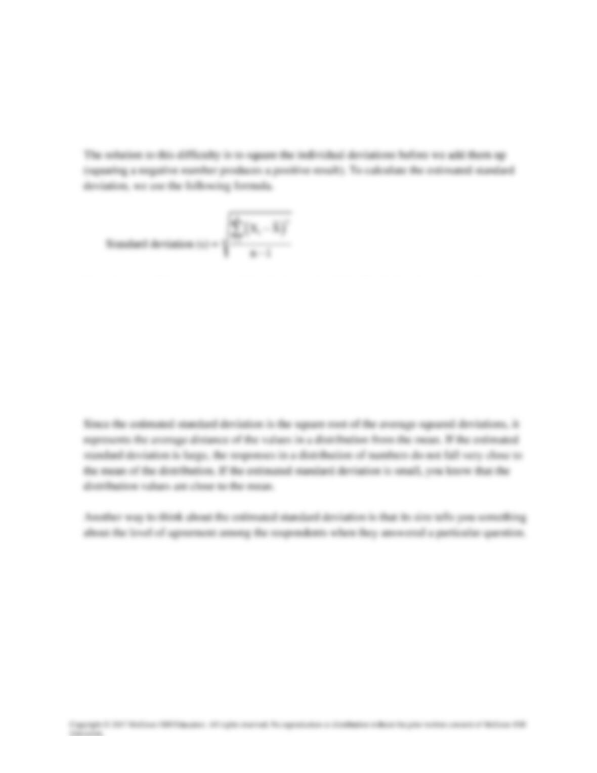
Once the sum of the squared deviations is determined, it is divided by the number of
respondents minus 1. The number 1 is subtracted from the number of respondents to help
produce an unbiased estimate of the standard deviation. The result of dividing the sum of the
squared deviations is the average squared deviation. To convert the result to the same units of
measure as the mean, we take the square root of the answer. This produces the estimated
standard deviation of the distribution. Sometimes the average squared deviation is also used as
a measure of dispersion for a distribution. The average squared deviation, called the variance,
is used in a number of statistical processes.
Together with the measures of central tendency, these descriptive statistics can reveal a lot
about the distribution of a set of numbers representing the answers to an item on a questionnaire.
Often, however, marketing researchers are interested in more detailed questions that involve
more than one variable at a time.
D. SPSS Applications—Measures of Dispersion (PPT slide 11-7)
The text uses the restaurant database with the SPSS software to calculate measures of
dispersion. Exhibit 11.3 shows the output for the measures of dispersion for variable
6
Chapter 11 – Basic Data Analysis for Quantitative Research
X22–Satisfaction. (PPT slide 11-7).
E. Preparation of Charts
Many types of charts and graphics can be prepared easily using the SPSS software. Charts and
other visual communication approaches should be used whenever practical. They help
information users to quickly grasp the essence of the results developed in data analysis, and also
can be an effective visual aid to enhance the communication process and add clarity and impact
to research reports and presentations.
II. How to Develop Hypotheses (PPT slide 11-8)
Measures of central tendency and dispersion are useful tools for marketing researchers. But
researchers often have preliminary ideas regarding data relationships based on the research
objectives. These ideas are derived from previous research, theory and/or the current business
situation, and typically are called hypotheses. A hypothesis is an unproven supposition or
proposition that tentatively explains certain facts or phenomena. A hypothesis also may be thought
of as an assumption about the nature of a particular situation. Statistical techniques enable us to
determine whether the proposed hypotheses can be confirmed by the empirical evidence.
7
Chapter 11 – Basic Data Analysis for Quantitative Research
null hypothesis. The alternative hypothesis is that there is a difference between the group means. If
the null hypothesis is accepted, there is no change in the status quo. But if the null hypothesis is
rejected and the alternative hypothesis accepted, the conclusion is there has been a change in
behavior, attitudes, or some similar measure.
III. Analyzing Relationships of Sample Data (PPT slide 11-9)
Marketing researchers often wish to test hypotheses about proposed relationships in the sample
data.
A. Sample Statistics and Population Parameters
The purpose of inferential statistics is to make a determination about a population on the basis
of a sample from that population.
A frequency distribution displaying the data obtained from the sample is commonly used to
summarize the results of the data collection process. When a frequency distribution displays a
variable in terms of percentages, then this distribution represents proportions within a
population. The proportion may be expressed as a percentage, a decimal value, or a fraction.
B. Choosing the Appropriate Statistical Technique
After the researcher has developed the hypotheses and selected an acceptable level of risk
(statistical significance), the next step is to test the hypotheses. To do so, the researcher must
select the appropriate statistical technique to test the hypotheses. A number of statistical
techniques can be used to test hypotheses. Several considerations influencing the choice of a
particular technique are given below.
• The number of variables
8
Chapter 11 – Basic Data Analysis for Quantitative Research
variables at the same time to represent the real world and fully explain relationships in the data.
In such cases, multivariate statistical techniques are required.
Exhibit 11.6 provides an overview of the types of scales used in different situations. With
ordinal data one can use only the median, percentile, and Chi-square.
After considering the measurement scales and data distributions, there are three approaches for
analyzing sample data that are based on the number of variables. One can use univariate,
bivariate, or multivariate statistics. Univariate statistics means one can statistically analyze only
one variable at a time. Bivariate analyzes two variables. Multivariate examines many variables
simultaneously.
C. Univariate Statistical Tests (PPT slide 11-10)
Univariate tests of significance are used to test hypotheses when the researcher wishes to test a
proposition about a sample characteristic against a known or given standard. The following are
some examples of propositions.
• The new product or service will be preferred by 80 percent of our current customers.
• The average monthly electric bill in Miami, Florida, exceeds $250.00.
One can translate these propositions into a null hypotheses and test them. Hypotheses are
developed based on theory, previous relevant experiences, and current market conditions.
The process of testing hypotheses regarding population characteristics based on sample data
often begins by calculating frequency distributions and averages, and then moves on to further
analysis that actually tests the hypotheses. When the hypothesis testing involves examining one
9
Chapter 11 – Basic Data Analysis for Quantitative Research
variable at a time, it is referred to as a univariate statistical test. When the hypothesis testing
involves two variables it is called a bivariate statistical test.
D. SPSS Application—Univariate Hypothesis Test (PPT slide 11-11)
Using the SPSS software, researchers can test the responses in the Santa Fe Grill database to
find the answer to the research questions posed above. The SPSS output is shown in Exhibit
11.8 (PPT slide 11-11).
E. Bivariate Statistical Tests (PPT slide 11-12)
In many instances marketing researchers test hypotheses that compare the characteristics of two
groups or two variables (PPT slide 11-12). There are three types of bivariate hypothesis tests:
F. Cross-Tabulation (PPT slide 11-13 and 11-14)
Cross-tabulation is useful for examining relationships and reporting the findings for two
variables. The purpose of cross tabulation is to determine if differences exist between
subgroups of the total sample. In fact, cross tabulation is the primary form of data analysis in
some marketing research projects. To use cross tabulation the researcher must understand how
to develop a cross tabulation table and how to interpret the outcome.
10
Chapter 11 – Basic Data Analysis for Quantitative Research
When constructing a cross tabulation table, the researcher selects the variables to use when
examining relationships. Selection of variables should be based on the objectives of the
research project and the hypotheses being tested. But in all cases remember that Chi-square is
the statistic to analyze nominal (count) or ordinal (ranking) scaled data. Paired variable
relationships (e.g., gender of respondent and ad recall) are selected on the basis of whether the
variables answer the research questions in the research project and are either nominal or ordinal
data.
Cross-tabulation provides the research analyst with a powerful tool to summarize survey data. It
is easy to understand and interpret and can provide a description of both total and subgroup data.
Yet the simplicity of this technique can create problems. It is easy to produce an endless variety
of cross tabulation tables. In developing these tables, the analyst must always keep in mind both
the project objectives and specific research questions of the study.
G. Chi-Square Analysis (PPT slide 11-15)
Chi-square (X2) analysis enables researchers to test for statistical significance between the
frequency distributions of two (or more) nominally scaled variables in a cross tabulation table
to determine if there is any association between the variables (PPT slide 11-15). Categorical
data from questions about sex, education, or other nominal variables can be tested with this
H. Calculating the Chi-Square Value (PPT slide 11-15)
The formula to calculate the Chi-square value is shown below.
11
Chapter 11 – Basic Data Analysis for Quantitative Research
Chi-square formula
( )
2
2
1
Observed Expected
xExpected
n
ii
ii
−
−
=
Where:
Observedi = observed frequency in cell i
Expectedi = expected frequency in cell i
n = number of cells
I. SPSS Application—Chi-Square
Based on their conversations with customers, the owners of the Santa Fe Grill believe that
female customers drive to the restaurant from farther away than do male customers. The
Chi-square statistic can be used to determine if this is true. The SPSS results are shown in
Exhibit 11.10.
J. Comparing Means: Independent Versus Related Samples (PPT slide 11-16)
In addition to examining frequencies, marketing researchers often want to compare the means
of two groups (PPT slide 11-16). In fact, one of the most frequently examined questions in
marketing research is whether the means of two groups of respondents on some attitude or
behavior are significantly different.
In a related sample situation, the marketing researcher must take special care in analyzing the
12
Chapter 11 – Basic Data Analysis for Quantitative Research
information. Although the questions are independent, the respondents are the same. This is
called a paired sample. When testing for differences in related samples the researcher must use
what is called a paired samples t-test.
K. Using the t-Test to Compare Two Means (PPT slide 11-17)
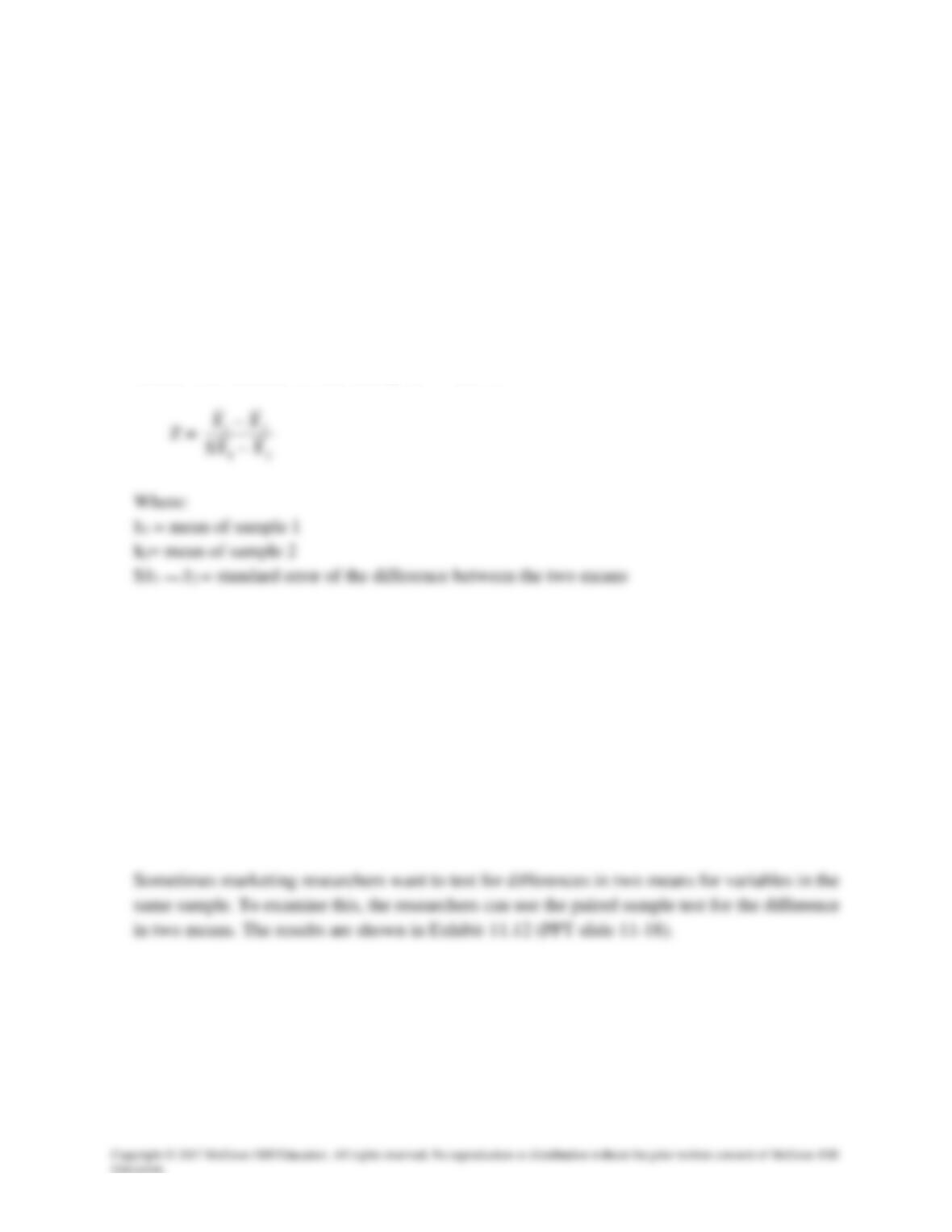
The t-test for differences between group means can be conceptualized as the difference
between the means divided by the variability of the means. The t value is a ratio of the
difference between the two sample means and the standard error. The t-test provides a
mathematical way of determining if the difference between the two sample means occurred by
chance. The formula for calculating the t value is:
L. SPSS Application—Independent Samples t–Test
To illustrate the use of a t-test for the difference between two group means, the text uses the
restaurant database. Based on their experiences observing customers in the restaurant the Santa
Fe Grill owners believe there are differences in the levels of satisfaction between male and
female customers. To test this hypothesis, researchers can use the SPSS “Compare Means”
program. The results are shown in Exhibit 11.11.
M. SPSS Application—Paired Samples t-Test (PPT slide 11-18)
N. Analysis of Variance (ANOVA) (PPT slide 11-19)
Researchers use analysis of variance (ANOVA) to determine the statistical difference between
three or more means.
One-way ANOVA is used to examine group means. The term one-way is used because the