
1
Part Six
Comprehensive Cases – Solutions
Table of Contents
Comprehensive Cases – Solutions ……………………………………………………………………. 1
Case 1 ………………………………………………………………………………………………………………..1
Case 2 ………………………………………………………………………………………………………………..8
Case 3 ………………………………………………………………………………………………………………..9
Case 4 ……………………………………………………………………………………………………………… 20
Case 5 ……………………………………………………………………………………………………………… 27
Case 6 ……………………………………………………………………………………………………………… 30
Case 7: Knowing the Way ……………………………………………………………………………………. 37
Case 1
Running the Numbers: Does It Pay?
Database: Students are instructed to download the data sets for this case from the book’s
Objectives: This case allows the student to consider the ethical dimension in marketing research,
to develop hypotheses, and to gain experience in how to test them.
Summary: Dr. William Ray, a research consultant, has received a government grant to research
how aspects of a student’s college experiences relate to his or her job performance. The grant is
RQ1: Does a student’s liking of quantitative coursework in college affect his or her future
earnings?

Comprehensive Case Solutions: Essentials of Marketing Research, 11th Edition,
Cengage. 2
RQ2: Do people with an affinity for quantitative courses get promoted more quickly than those
who do not?
Questions
1. Does the grant present Dr. Ray with an ethical dilemma?
2. Derive at least one hypothesis for each research question listed above.
While students’ hypotheses will differ, possible hypotheses for RQ1 could be:
or
or
As long as the students provide a reasonable rationale, they should be credit for doing so. One
possible line of thought is that those students who like quantitative subject matter may tend to
Possible hypotheses for RQ2 could be:
or
Cengage. 3
While students could pick out individual items to serve as proxy variables for testing hypotheses
like those raised above, students, particularly more advanced students, will try to apply composite
Factor Analysis: A factor analysis is not necessary — but it can be used by advanced students
(particularly those using Exploring Marketing Research as opposed to Essentials of Marketing
Research) to examine scale validity. The factor results also show which items may need to be
recoded based on the opposing sign of a loading estimate. Otherwise, the content of the item
and/or the pattern of correlations among the items would suggest the same. In this case, X3
Total Variance Explained
Component
Initial Eigenvalues
Extraction Sums of Squared Loadings
Total
% of Variance
Cumulative %
Total
% of Variance
Cumulative %
1
3.118
62.365
62.365
3.118
62.365
62.365
2
.680
13.606
75.971
3
.590
11.808
87.779
4
.449
8.985
96.764
5
.162
3.236
100.000
Extraction Method: Principal Component Analysis.
Component Matrix(a)
Component
1
x1
.936
x2
.680
x3
-.720
x4
.767
x5
-.821
Extraction Method: Principal Component Analysis.
a 1 components extracted.
Reliability: Alpha computed for multi-item scale … it is .84 — acceptable.
Reliability Statistics
Cronbach’s
Alpha
N of Items
Cengage. 4
.839
5
Item-Total Statistics
Scale Mean if
Item Deleted
Scale Variance
if Item Deleted
Corrected
Item-Total
Correlation
Cronbach’s
Alpha if Item
Deleted
x1
12.09
13.584
.867
.746
x2
12.54
15.607
.526
.838
x3
12.92
15.034
.569
.828
x4
11.98
14.194
.614
.817
x5
12.24
15.300
.681
.799
3. Use the data that correspond to the case to perform a test of each hypothesis created. The
material in the front of chapter 15, around pages 412 – 415, should be particularly helpful.
The following descriptions illustrate some example hypotheses and tests of those hypotheses.
Student responses may vary. Instructors should be mindful of the level of students in the
expectations of the analytical rigor applied in testing the hypotheses.
Regression: H2a: Students attitude toward math is related positively to their salary
potential: Supported (using simple regression below and a positive and significant
regression coefficient – a correlation coefficient would also be acceptable).
Model Summary
Model
R
R Square
Adjusted R
Square
Std. Error of
the Estimate
1
.200(a)
.040
.037
$10,388.492
a Predictors: (Constant), LikeMath
ANOVA(b)
Model
Sum of Squares
df
Mean Square
F
Sig.
1
Regression
1333679368.547
1
1333679368.547
12.358
.001(a)
Residual
32160387123.832
298
107920762.161
Total
33494066492.379
299
a Predictors: (Constant), LikeMath
b Dependent Variable: SALARY
Coefficients(a)
Model
Unstandardized Coefficients
Standardized Coefficients
Sig.
B
Std. Error
Beta
t
1
(Constant)
29843.887
2060.720
14.482
.000
LikeMath
448.776
127.661
.200
3.515
.001
Comprehensive Case Solutions: Essentials of Marketing Research, 11th Edition,
Cengage. 5
a Dependent Variable: SALARY
H2b: Those employees who get promoted will report a more positive attitude toward math than
those employees who do not get promoted.
Using the summed scale for attitudes described above, one can use an independent samples t–
test to examine the hypothesis because the outcome (promotion) is a nominal grouping variable
At first glance, using a 0.1 type I error rate (), the hypothesis would be supported because those
who are promoted have a statistically significant higher average (16.2 versus 15.2). However, if
the type I error rate is less than 0.1, say 0.05, the hypothesis is not supported. Strictly speaking,
the hypothesis is directional (implies more than a relationship but also the direction of the
relationship – “a more positive attitude” is predicted for promoted employees). In this case, a
4. Is there evidence supporting the discrimination claim? Explain.
5. List another hypothesis (unrelated to the research questions in the grant) that could be tested
Cengage. 6
There are many hypotheses that students could come up with. One may involve whether or
not GPA is related to salary (if you wish to assign them this specific hypotheses, feel free to
do so to reduce the flexibility in responses). For example:
6. Test the hypothesis developed in 5.
Given that both of these variables are continuous, either correlation or simple regression
could be used to test that hypothesis.
7. Considering employees’ aptitudes about their college experience, does the amount of fun
that students had in college or the degree to which they thought quant classes were a positive
experience relate more strongly to salary?
Summated (composite) constructs for both the X (Enjoy Math Courses) and S (Fun at College)
variables will be useful here again. Also here, S5 turns out to not correlate highly with S1-S4
as indicated by the coefficient alpha program or factor analysis or just item-correlations.
Students should not use S5 as part of the scale. Thus, the composite consists of only S1-S4.
8. Would the “problem” that led to the grant be a candidate for ethnographic research? Explain.

Case 2
Good Times at GoodBuy?
Overview: This case provides students with a good opportunity to perform basic types
of procedures and analysis associated with typical survey-based marketing/market
research. The data contains several opportunities to create scales and to examine the
measurement validity associated with each. For advanced students, the data provide a
good opportunity to employ advanced analytical tools including multivariate data
analysis. For less advanced students, limit the questions to the first three (numbers 1 –
3 as included in Essentials of Marketing Research).
1. Are the data appropriate for multiple regression analysis? If so, what
technique(s) would you suggest as appropriate and why?
2. The researcher suggests that you first use only half of the data to do an initial
analysis (split the entire sample randomly into two halves of 200 respondents
each). Do you think that is a good idea? Explain.
Case 3
Attiring Situation
Database: Students should download this data from cengagebrain.com using the student
resources associated with this book.
Objectives: This case allows the student to create hypotheses and conduct statistical analyses to
Summary: RESERV is a national placement firm specializing in putting retailers and service
providers together with potential employees who fill positions at all levels of the organization—
from entry-level positions to senior management positions. One specialty clothing store chain
A laboratory experiment is designed in which two variables are manipulated in a between-
subjects design: employee attire (professional/unprofessional) and manner with which the
employee tries to gain extra sales (soft close/hard close). Subjects’ biological sex was recorded
The experiment was conducted in a university union, and subjects were recruited to participate
as customers who had just purchased some dress slacks and a shirt in a mock retail environment.
The employee was to complete the transaction and try to sell the customer some of several
accessory items displayed at the counter. Each subject was randomly assigned to one of four
conditions where the employee was either:

2. Dressed unprofessionally and used a soft close.
4. Dress unprofessionally and used a hard close.
The researcher wishes to use this information to explain how employee appearance encourages
shoppers to continue shopping (TIME) and spend money (SPEND). Each subject was given $25 (in
Questions
1. Develop at least three hypotheses that correspond to the research questions.
Students’ hypotheses may vary (if you do not want them to vary – assign the hypotheses below).
However, some possible hypotheses are:
2. Test the hypotheses using an appropriate statistical approach. The introductory materials of
Chapters 14 and 15 should be useful in choosing an appropriate statistic.
The appropriate statistical approach will depend on the hypotheses students develop. ANOVA is
a very appropriate statistical approach for the hypotheses given above.
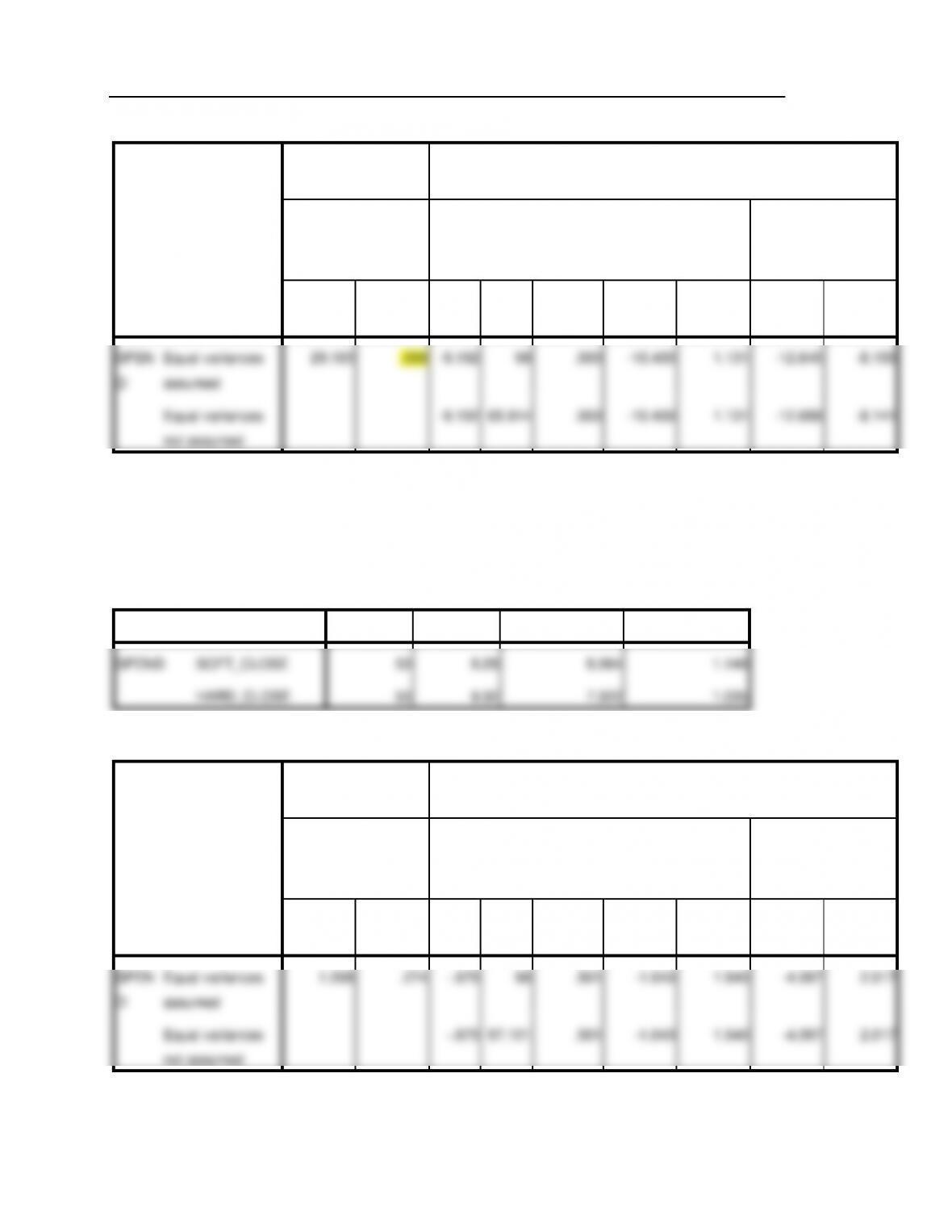
To test H1 above, ANOVA is appropriate:
Group Statistics
X1
N
Mean
Std. Deviation
Std. Error Mean
SPEND
PROF_ATTIRE
50
3.60
3.110
.440
UNPROF_ATTIRE
50
14.00
7.371
1.042
Comprehensive Case Solutions: Essentials of Marketing Research, 11th Edition,
Cengage. 11
Independent Samples Test
Levene’s Test for
Equality of Variances
t-test for Equality of Means
95% Confidence
Interval of the
Difference
F
Sig.
t
df
Sig. (2-
tailed)
Mean
Difference
Std. Error
Difference
Lower
Upper
SPEN
D
Equal variances
assumed
29.103
.000
-9.192
98
.000
-10.400
1.131
-12.645
-8.155
Equal variances
not assumed
-9.192
65.914
.000
-10.400
1.131
-12.659
-8.141
These results suggest that customers spend less when the employee is dressed professionally,
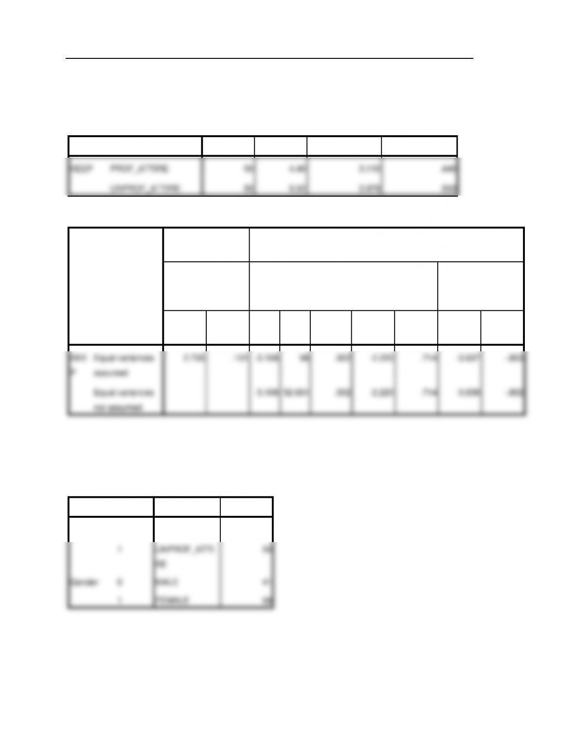
providing support for H1. However, there is no significant different on the amount spend due to
the type of close used by the employee (H2):
Group Statistics
X2
N
Mean
Std. Deviation
Std. Error Mean
SPEND
SOFT_CLOSE
50
8.28
8.064
1.140
HARD_CLOSE
50
9.32
7.322
1.035
Independent Samples Test
Levene’s Test for
Equality of Variances
t-test for Equality of Means
95% Confidence
Interval of the
Difference
F
Sig.
t
df
Sig. (2-
tailed)
Mean
Difference
Std. Error
Difference
Lower
Upper
SPEN
D
Equal variances
assumed
1.208
.274
-.675
98
.501
-1.040
1.540
-4.097
2.017
Equal variances
not assumed
-.675
97.101
.501
-1.040
1.540
-4.097
2.017
Comprehensive Case Solutions: Essentials of Marketing Research, 11th Edition,
Cengage. 12
Similarly, the results do not support H3, which hypothesized that customers would keep less
money if the employee was dressed professionally. There was no significant difference on how
much money customers kept due to the employee’s attire:
Group Statistics
X1
N
Mean
Std. Deviation
Std. Error Mean
KEEP
PROF_ATTIRE
50
4.40
3.110
.440
UNPROF_ATTIRE
50
6.62
3.979
.563
Independent Samples Test
Levene’s Test for
Equality of Variances
t-test for Equality of Means
95% Confidence
Interval of the
Difference
F
Sig.
t
df
Sig. (2-
tailed)
Mean
Difference
Std. Error
Difference
Lower
Upper
KEE
P
Equal variances
assumed
2.735
.101
-3.108
98
.002
-2.220
.714
-3.637
-.803
Equal variances
not assumed
-3.108
92.601
.002
-2.220
.714
-3.638
-.802
Finally, H4 stated that males would spend less than females if the employee was dressed
professionally, which is supported by the results given below:
Between-Subjects Factors
Value Label
N
X1
0
PROF_ATTIRE
50
1
UNPROF_ATTI
RE
50
Gender
0
MALE
41
1
FEMALE
59
Cengage. 13
Tests of Between-Subjects Effects
Dependent Variable:SPEND
Source
Type III Sum of
Squares
df
Mean Square
F
Sig.
Corrected Model
2988.385a
3
996.128
33.535
.000
Intercept
6750.794
1
6750.794
227.266
.000
X1
2112.722
1
2112.722
71.125
.000
Gender
25.206
1
25.206
.849
.359
X1 * Gender
220.312
1
220.312
7.417
.008
Error
2851.615
96
29.704
Total
13584.000
100
Corrected Total
5840.000
99
a. R Squared = .512 (Adjusted R Squared = .496)
EXP1 * Gender
Dependent Variable:SPEND
EXP1
Gender
Mean
Std. Error
95% Confidence Interval
Lower Bound
Upper Bound
PROF_ATTIRE
MALE
1.871
.979
-.072
3.814
FEMALE
6.421
1.250
3.939
8.903
UNPROF_ATTIRE
MALE
15.800
1.723
12.379
19.221
FEMALE
13.550
.862
11.839
15.261
3. Suppose the researcher is curious about how the feelings captured with the semantic
differentials influence the dependent variables SPEND and KEEP. Conduct an analysis to
explore this possibility. Are any problems present in testing this?
Comprehensive Case Solutions: Essentials of Marketing Research, 11th Edition,
Cengage. 14
Variables Entered/Removed
Model
Variables Entered
Variables
Removed
Method
1
SD8, SD2, SD1,
SD5, SD3, SD7,
SD4, SD6a
.
Enter
a. All requested variables entered.
Model Summary
Model
R
R Square
Adjusted R Square
Std. Error of the
Estimate
1
.231a
.053
-.033
7.805
a. Predictors: (Constant), SD8, SD2, SD1, SD5, SD3, SD7, SD4, SD6
ANOVAb
Model
Sum of Squares
df
Mean Square
F
Sig.
1
Regression
302.072
8
37.759
.620
.759a
Residual
5360.958
88
60.920
Total
5663.030
96
a. Predictors: (Constant), SD8, SD2, SD1, SD5, SD3, SD7, SD4, SD6
b. Dependent Variable: SPEND
Comprehensive Case Solutions: Essentials of Marketing Research, 11th Edition,
Cengage. 15
Coefficientsa
Model
Unstandardized Coefficients
Standardized
Coefficients
t
Sig.
Collinearity Statistics
B
Std. Error
Beta
Tolerance
VIF
1
(Constant)
39.430
15.430
2.555
.012
SD1
.441
.436
.117
1.012
.314
.809
1.236
SD2
-.067
.718
-.018
-.094
.926
.289
3.456
SD3
-1.184
1.030
-.311
-1.150
.253
.147
6.789
SD4
-2.570
1.772
-.647
-1.450
.150
.054
18.496
SD5
-.771
1.100
-.159
-.701
.485
.209
4.778
SD6
-3.325
1.927
-.837
-1.726
.088
.046
21.871
SD7
.124
1.856
.021
.067
.947
.109
9.147
SD8
-.283
1.161
-.052
-.244
.808
.237
4.216
a. Dependent Variable: SPEND
Collinearity Diagnosticsa
Model
Dime
nsion
Eigenvalu
e
Condition
Index
Variance Proportions
(Constant)
SD1
SD2
SD3
SD4
SD5
SD6
SD7
SD8
1
1
7.750
1.000
.00
.00
.00
.00
.00
.00
.00
.00
.00
2
.899
2.936
.00
.00
.01
.01
.00
.00
.00
.00
.00
3
.165
6.857
.00
.84
.01
.00
.00
.00
.00
.00
.01
4
.084
9.612
.00
.01
.02
.00
.00
.02
.01
.01
.18
5
.055
11.825
.00
.01
.72
.21
.00
.00
.00
.00
.00
6
.022
18.767
.01
.01
.07
.27
.11
.44
.04
.00
.00
7
.017
21.616
.00
.08
.11
.33
.22
.51
.05
.02
.00
8
.007
33.596
.00
.00
.03
.01
.02
.01
.12
.93
.77
9
.002
64.973
.99
.04
.02
.16
.64
.01
.77
.04
.04
a. Dependent Variable: SPEND
Comprehensive Case Solutions: Essentials of Marketing Research, 11th Edition,
Cengage. 16
Variables Entered/Removed
Model
Variables Entered
Variables
Removed
Method
1
SD8, SD2, SD1,
SD5, SD3, SD7,
SD4, SD6a
.
Enter
a. All requested variables entered.
Model Summary
Model
R
R Square
Adjusted R Square
Std. Error of the
Estimate
1
.185a
.034
-.054
3.823
a. Predictors: (Constant), SD8, SD2, SD1, SD5, SD3, SD7, SD4, SD6
ANOVAb
Model
Sum of Squares
df
Mean Square
F
Sig.
1
Regression
45.408
8
5.676
.388
.924a
Residual
1285.977
88
14.613
Total
1331.384
96
a. Predictors: (Constant), SD8, SD2, SD1, SD5, SD3, SD7, SD4, SD6
b. Dependent Variable: KEEP
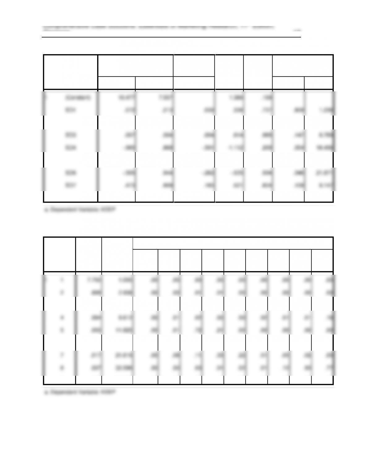
Cengage. 17
Coefficientsa
Model
Unstandardized Coefficients
Standardized
Coefficients
t
Sig.
Collinearity Statistics
B
Std. Error
Beta
Tolerance
VIF
1
(Constant)
10.477
7.557
1.386
.169
SD1
.072
.213
.039
.336
.737
.809
1.236
SD2
.193
.352
.107
.549
.584
.289
3.456
SD3
.007
.504
.004
.014
.989
.147
6.789
SD4
-.965
.868
-.501
-1.112
.269
.054
18.496
SD5
-.402
.539
-.171
-.746
.458
.209
4.778
SD6
-.505
.944
-.262
-.535
.594
.046
21.871
SD7
.473
.909
.165
.521
.604
.109
9.147
SD8
-.113
.569
-.043
-.200
.842
.237
4.216
a. Dependent Variable: KEEP
Collinearity Diagnosticsa
Mode
l
Dime
nsion
Eigenvalu
e
Condition
Index
Variance Proportions
(Constant
)
SD1
SD2
SD3
SD4
SD5
SD6
SD7
SD8
1
1
7.750
1.000
.00
.00
.00
.00
.00
.00
.00
.00
.00
2
.899
2.936
.00
.00
.01
.01
.00
.00
.00
.00
.00
3
.165
6.857
.00
.84
.01
.00
.00
.00
.00
.00
.01
4
.084
9.612
.00
.01
.02
.00
.00
.02
.01
.01
.18
5
.055
11.825
.00
.01
.72
.21
.00
.00
.00
.00
.00
6
.022
18.767
.01
.01
.07
.27
.11
.44
.04
.00
.00
7
.017
21.616
.00
.08
.11
.33
.22
.51
.05
.02
.00
8
.007
33.596
.00
.00
.03
.01
.02
.01
.12
.93
.77
9
.002
64.973
.99
.04
.02
.16
.64
.01
.77
.04
.04
a. Dependent Variable: KEEP
4. Critique the experiment from an internal and external validity viewpoint.
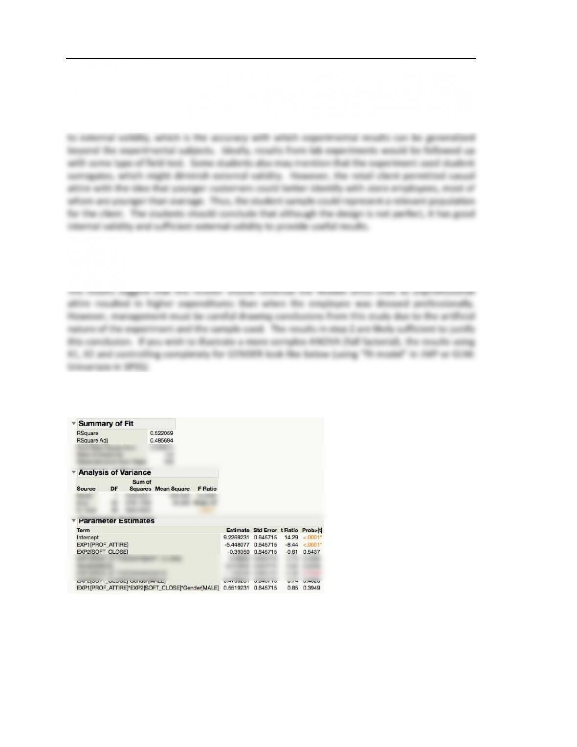
Comprehensive Case Solutions: Essentials of Marketing Research, 11th Edition,
Cengage. 18
The approach used a laboratory experiment, which allows the researcher more complete control
over the research setting and extraneous variables. Thus, the experiment has high internal
validity, which was defined in chapter 9 as the extent that an experimental variable is truly
responsible for any variance in the dependent variable. However, there is a tradeoff with respect
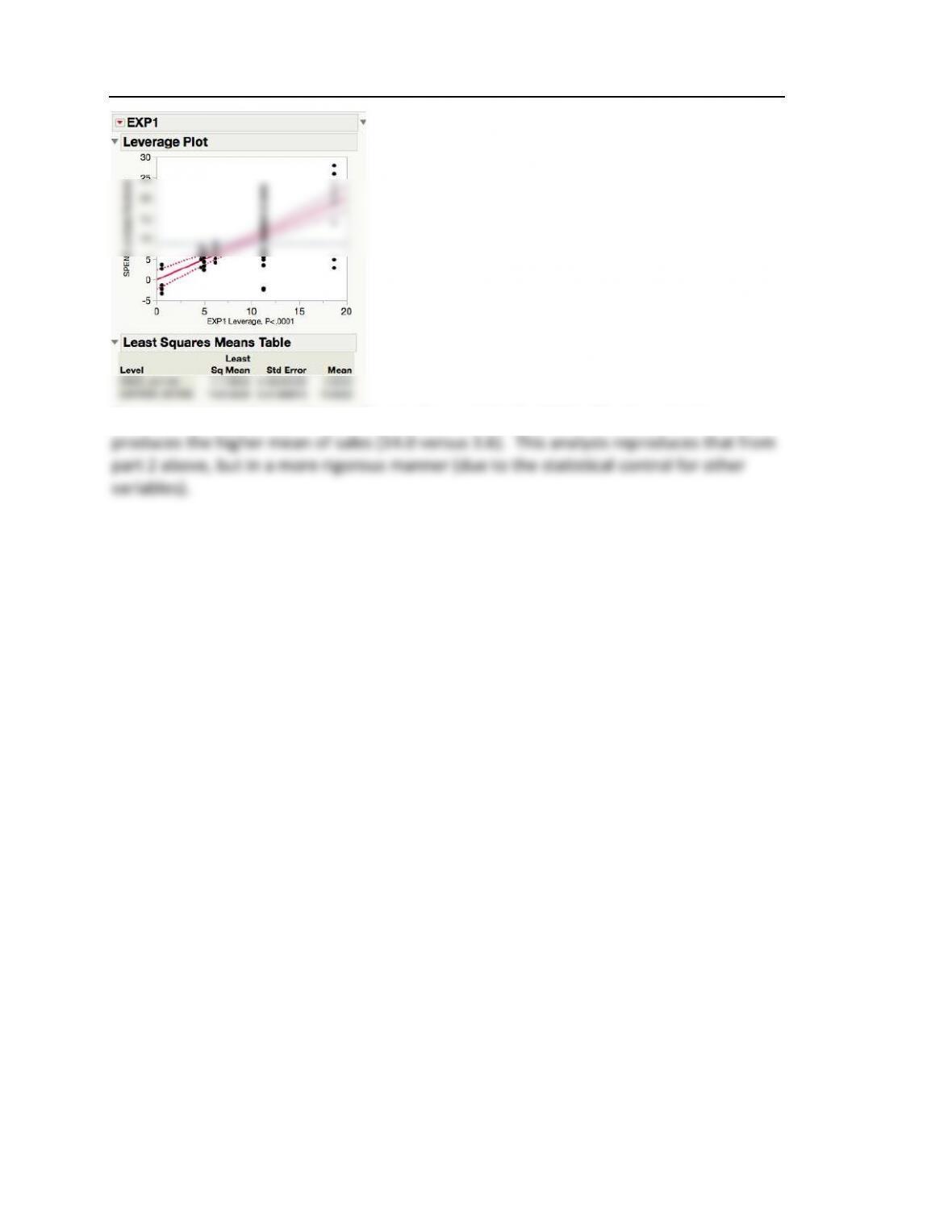
6. What conclusions would be justified by management regarding their employee appearance
policy?
Comprehensive Case Solutions: Essentials of Marketing Research, 11th Edition,
Cengage. 19
The only statistically significant effect in the model is for EXP1. The Casual attire

Case 4
Values and the Automobile Market
Database: Students are instructed to download the data for cases from the student resources
Objectives: The purpose of this case is to allow students to evaluate an entire research project.
Summary: During the 1990s, the luxury car segment became one of the most competitive in the
automobile market. Many American consumers who purchased luxury cars preferred imports
from Germany and Japan.
Questions:
1. Is the sampling method adequate? Is the attitude measuring scale sound? Explain.
2. Using the computerized database with a statistical software package, calculate the
means of the three automotive groups for the values variable. Do any of the values variables
show significant differences between American, Japanese, and European car owners?