Management Supplement A Homework This Situation Represents The Probability Type Error

Unlock access to all the studying documents.

View Full Document

Control charts are defined by the center line, upper control limit, and lower control

limit. These values are related to the expected value and variance of the statistics plot-

ted on the charts. In Chapter 12, the upper and lower control limits were specified

through the use of certain constants given in Appendix B. This section shows how

these factors are developed and discusses the statistical basis for the rules used to in-

terpret control charts.

Variables Control Charts

Under this assumption, 100(1 – α) percent of the sample means fall between µ–

zα/2σx

–and µ+ zα/2σx

–; these values become the lower and upper control limits. A value

of zα/2 = 3 gives a six-standard deviation range with α/2 = 0.0014. Thus, only about

0.3 percent of the sample observations will be expected to fall outside these limits. If

the process is in control, the likelihood that a sample will fall outside the control lim-

its is extremely small. On the other hand, if the true mean has shifted, this probabil-

ity will be much larger. This reasoning is the theoretical basis for assigning three-

sigma control limits.

Chapter 12 Statistical Process Control 757

HAPTER

12 A

PPENDIX

TATISTICAL

OUNDATIONS OF

ONTROL

HARTS



12Evans/final 5/4/01 11:23 AM Page 757

Note to reader: this appendix is drawn from the 5th edition; references to chapter 12

apply to Chapter 8 in this edition.

760 Part 3 Technical Issues in Quality

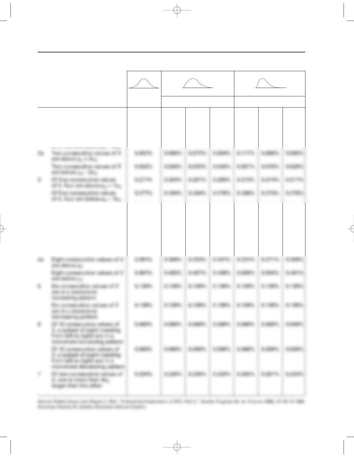
Table 12A.1 Rule Probabilities for x

–Charts When the Process Is in Control

Probability (sensitivity)

xis normal xis slightly skewed xis seriously skewed

Sample size Sample size

Sample size

Rule Description is irrelevant 5 10 25 5 10 25

–is more than 3σx

–above µx

–0.135% 0.254% 0.209% 0.191% 0.488% 0.380% 0.281%

–is more than 3σx

–below µx

–0.135% 0.021% 0.046% 0.080% 0.000% 0.008% 0.035%

2 Of three consecutive values 0.153% 0.237% 0.212% 0.190% 0.342% 0.281% 0.235%

of x

–, two are above µx

–+ 2σx

–

Of three consecutive values 0.153% 0.076% 0.098% 0.119% 0.020% 0.048% 0.082%

–, two are below µx

–– 2σx

–

3a Four consecutive values of x

–0.063% 0.065% 0.064% 0.064% 0.063% 0.063% 0.063%

are above µx

–+ 1σx

–

Four consecutive values of x

–0.063% 0.065% 0.065% 0.064% 0.061% 0.063% 0.063%

are below µx

––1σx

–

4 Seven consecutive values 0.781% 0.631% 0.680% 0.705% 0.494% 0.568% 0.636%

of x

–are above µx

–

Seven consecutive values 0.781% 0.961% 0.896% 0.865% 1.202% 1.060% 0.953%

of x

–are below µx

–

12Evans/final 5/4/01 11:23 AM Page 760

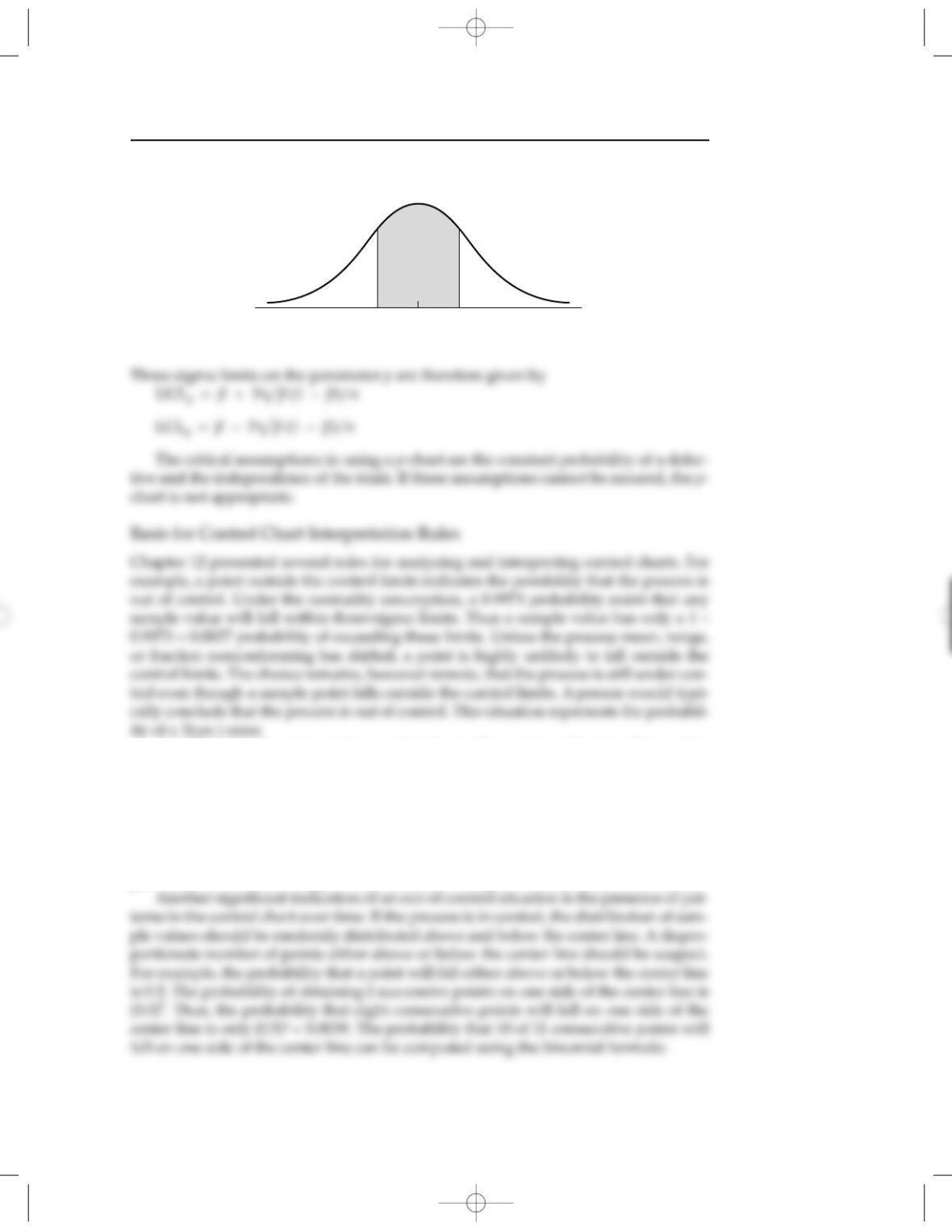
A second rule for interpreting control charts discussed in Chapter 12 was that

about two-thirds of the points should fall within the middle one-third of the region

between the control limits. This rule follows from the normality assumption that

about 68 percent of a normal distribution falls within one standard deviation on ei-

ther side of the mean (see Figure 12A.1). Therefore, if the process is in control and all

samples are chosen from a common population, this assumption should be true. If,

however, the value of the population parameter has shifted, the distribution of sam-

ple statistics will also change. In such a case, an assignable cause needs to be found.

68%

µ – σ µ µ + σ

Figure 12A.1 Area Under the Normal Curve

Within One Standard Deviation of the Mean

Chapter 12 Statistical Process Control 759

12Evans/final 5/4/01 11:23 AM Page 759

The expected value of Ris estimated by the sample range R

–. Thus R

–/d2is an esti-

mate of the process standard deviation σx. To establish control limits for an R-chart,

an estimate of the standard deviation of the random variable R, namely σR, is needed.

From the distribution of the statistic R/σx, the ratio σR/σxcan be computed for each

n, resulting in another constant d3.

For convenience, the constants 1 + 3d3/d2and 1 – 3d3/d2are computed as D4and D3,

respectively. The control limits for the R-chart are therefore based on the distribution

of the process standard deviation, adjusted to correspond to the range.

–-Chart The statistic x

–

–is an estimate of the population mean µ. Because R

–/d2is an es-

timate of σx, an estimate of the sample standard deviation is

Letting A2= 3/d2nprovides the control limits presented in Chapter 12:

UCLx

_=x

–

–+ A2R

–

LCLx

_=x

–

–– A2R

–

758 Part 3 Technical Issues in Quality

12Evans/final 5/4/01 11:23 AM Page 758

1. Robert W. Hoyer and Wayne C. Ellis, “A

Graphical Exploration of SPC, Part 1,” Quality

Progress 29, no. 5 (May 1996), 65–73.

2. This discussion is adapted from James R.

Evans, Statistical Process Control for Quality Improve-

5. Raymond R. Mayer, “Selecting Control Lim-

its,” Quality Progress 16, no 9, (1983), 24–26.

6. Robert W. Traver, “Pre-Control: A Good Al-

ternative to x– R-Charts,” Quality Progress 18, no. 9

(September 1985).

Chapter 12 Statistical Process Control 761

f(10) = 

(0.5)10(0.5)1= 0.00537

If the process is in control, either of these events is highly unlikely.

Table 12A.1 shows the probabilities associated with seven common rules used for

interpreting control charts for normal, slightly skewed, and seriously skewed process

outputs. Note that, even for the skewed distributions, almost all of the conditions

have probabilities less than 0.01 when the process is in control. Close analysis of this

table suggests the following:

NOTES

12Evans/final 5/4/01 11:23 AM Page 761