CHAPTER 9
Transportation and Assignment Models
TEACHING SUGGESTIONS
Teaching Suggestion 9.1: Transportation Models in the Chapter.
The linear programming approaches and the algorithmic approaches are used for bot the trans-
portation problem and the assignment problem. The instructor can choose to either of these
methods.
Teaching Suggestion 9.2: Using the Northwest Corner Rule.
This approach is easily understood by students and is appealing to teach for that very reason.
Teaching Suggestion 9.3: Using the Stepping-Stone Method.
Students usually pick up the concept of a closed path and learn to trace the pluses and minuses
Teaching Suggestion 9.4: Dummy Rows and Columns.
Another confusing issue to students is whether to add a dummy row (source) or dummy column
Teaching Suggestion 9.5: Handling Degeneracy in Transportation Problems.
Just as a warning, be aware that students are often confused by the concept of where to place the
zero so that the closed paths can be traced. Carefully explain why you chose or didn’t choose a
certain cell. The choice of cell can affect the number of iterations that follow.
Teaching Suggestion 9.6: Facility Location Problems.
These are an important application of the transportation model and make it easy to compare how
Teaching Suggestion 9.7: Sensitivity Analysis on the Assignment Problem.
This algorithm is easy to use and understand. Tell about solving a large staffing problem, then
Teaching Suggestion 9.8: Maximizing Assignment Problems.
This section is needed if students are to solve maximization problems by hand, but QM for Win-
Teaching Suggestion 9.9: Problem 9-46.
In assigning this challenging aggregate planning problem, you may wish to first provide some
background information on how to structure the plan. Remind students that back ordering is not
permitted, so very large costs must be inserted in many cells. Note that Problem 9-30 (Mehta
Company) is a warm-up exercise for this data set problem.
ALTERNATIVE EXAMPLES
Alternative Example 9.1: Let us presume that a product is made at two of our factories that we
wish to ship to three of our warehouses. We produce 18 at factory A and 22 at factory B; we
want 10 in warehouse 1, 20 in warehouse 2, and 10 in warehouse 3. Per unit transportation costs
are A to 1, $4; A to 2, $2; A to 3, $3; B to 1, $3; B to 2, $2; B to 3, $1. The corresponding trans-
portation table is
TO
Warehouses
FROM
1
2
3
Total
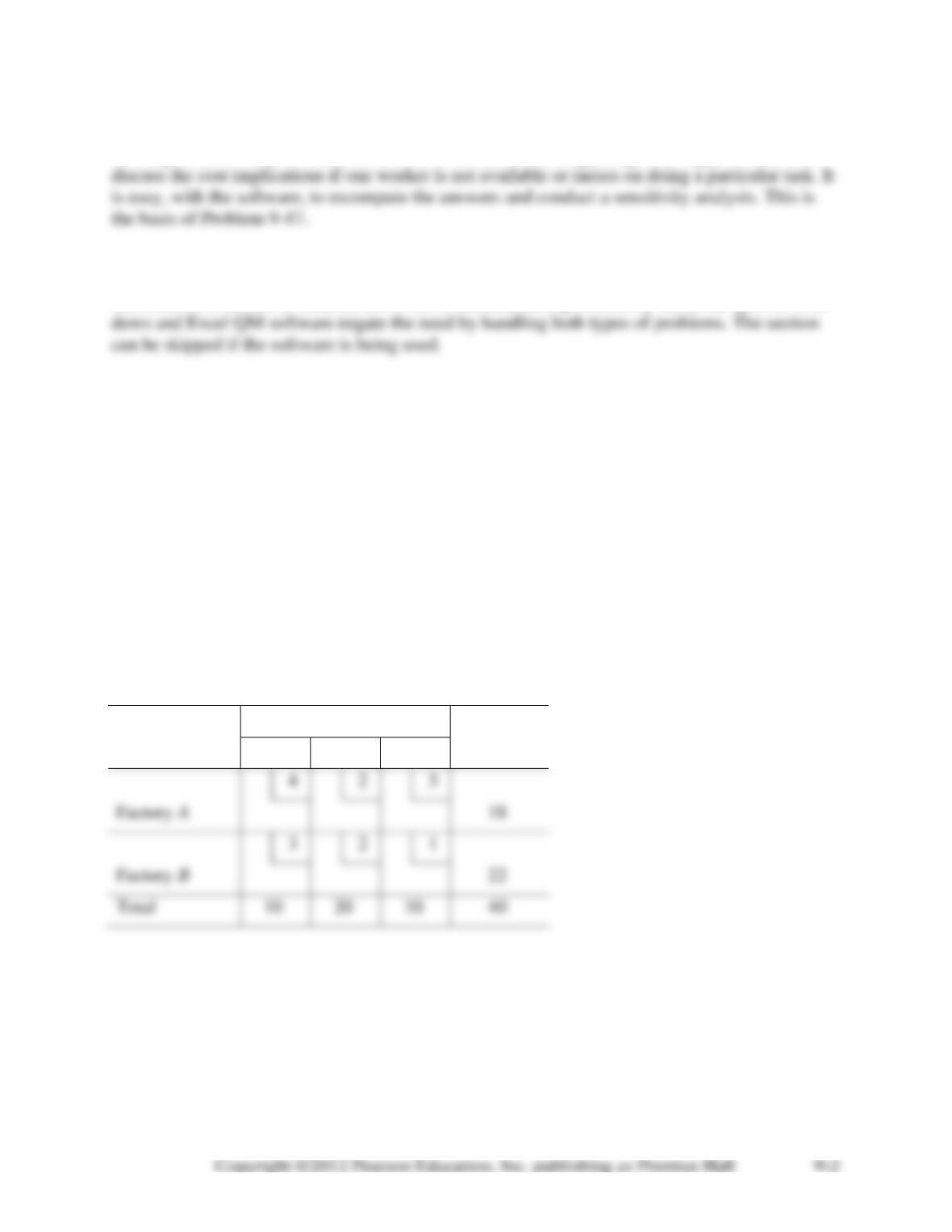
The northwest corner approach follows:
TO
Warehouses
FROM
1
2
3
Total
Factory A
4
2
3
18
10
8
Factory B
3
2
1
22
12
Total
10
20
Using the stepping-stone method, we can find the optimal solution:
SOLUTION:
TO
Warehouses
FROM
1
2
3
Total
Factory B
22
Total
10
20
10
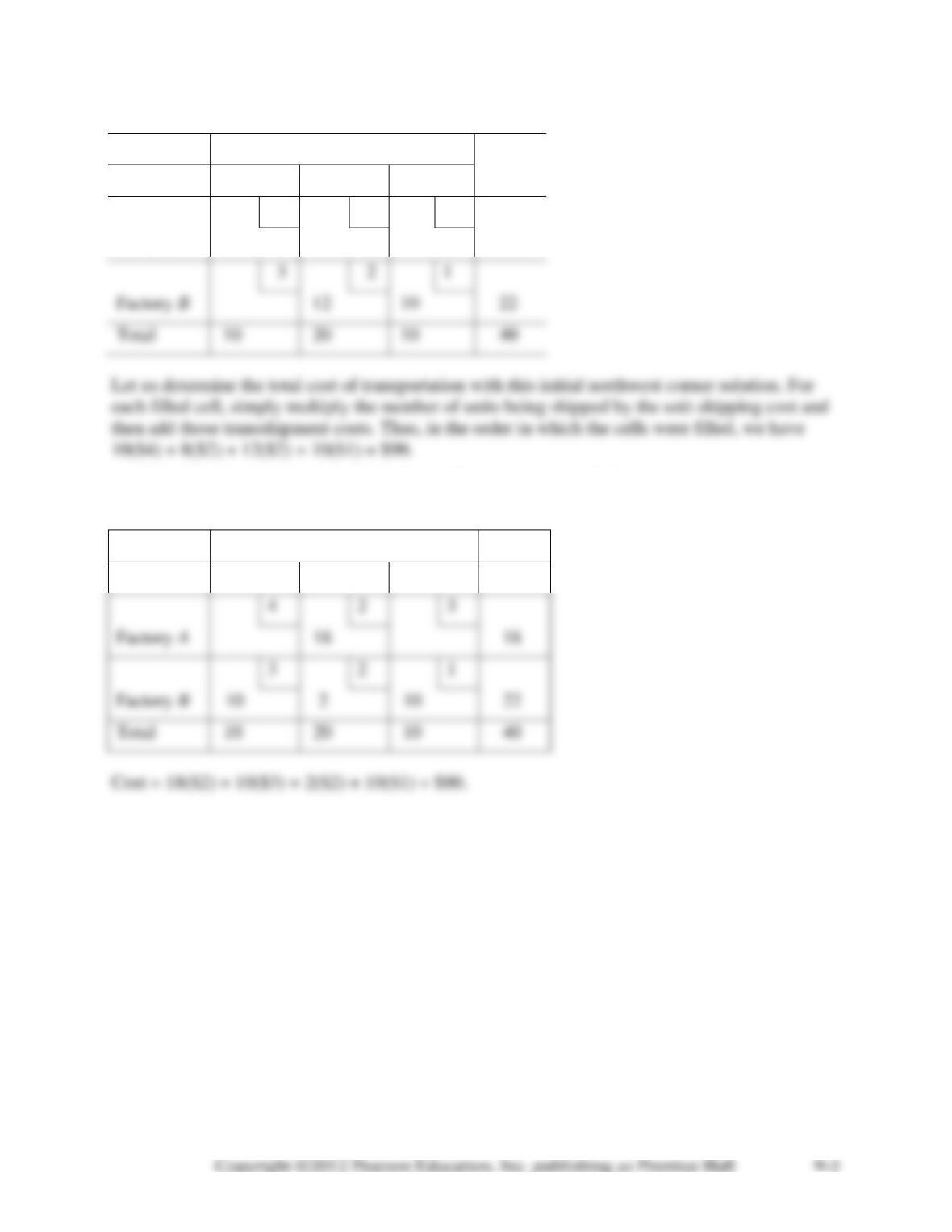
Alternative Example 9.2: There is often an imbalance between the amounts produced and the
amounts desired in the warehouses. In Alternative Example 9.1, there were 40 units produced
and forty units demanded for warehousing. Let us presume that an additional 4 units are desired
TO
Warehouses
FROM
1
2
3
Total
Factory A
4
2
3
14
4
18
Factory B
3
2
1
20
2
22
0
0
0
12
Total
14
24
14
52
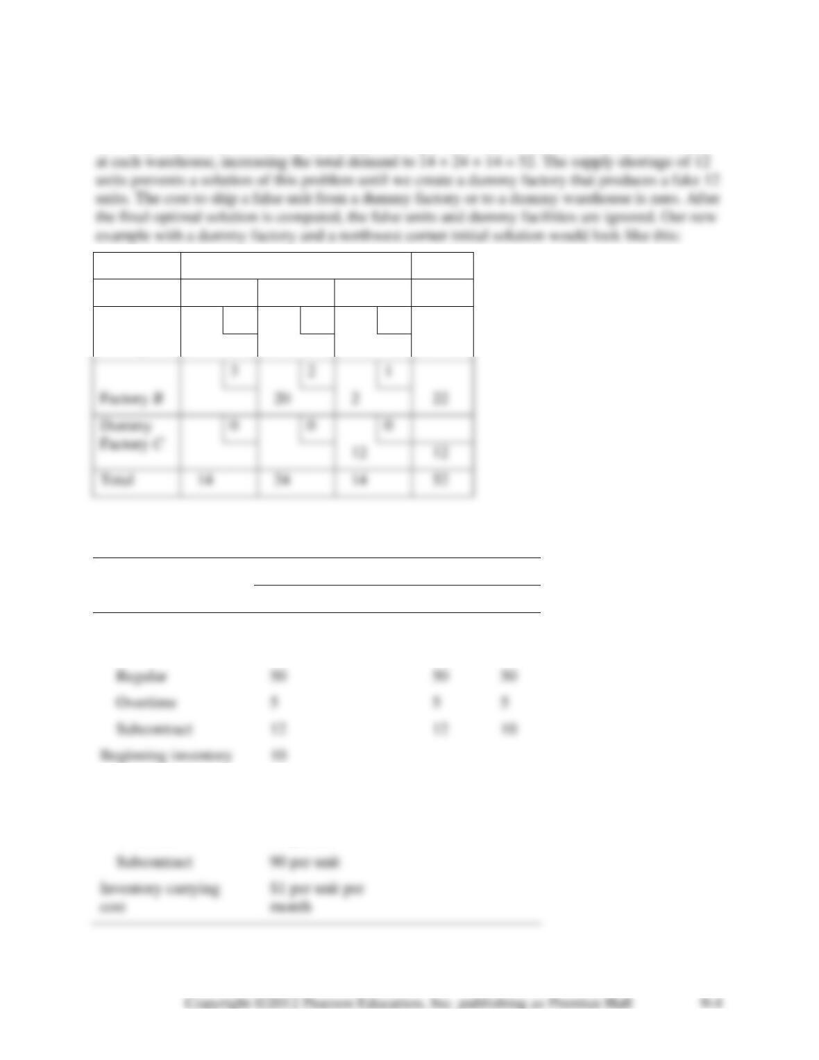
Alternative Example 9.3: Here is a production application of the transportation problem. Set up
the following problem in a transportation format and solve for the minimum-cost plan:
PERIOD
Feb
Mar
Apr
Demand
55
70
75
Capacity
Regular
50
50
50
Overtime
5
5
Subcontract
12
12
10
Beginning inventory
10
Costs
Regular time
$60 per unit
Overtime
80 per unit
Subcontract
90 per unit
cost
month
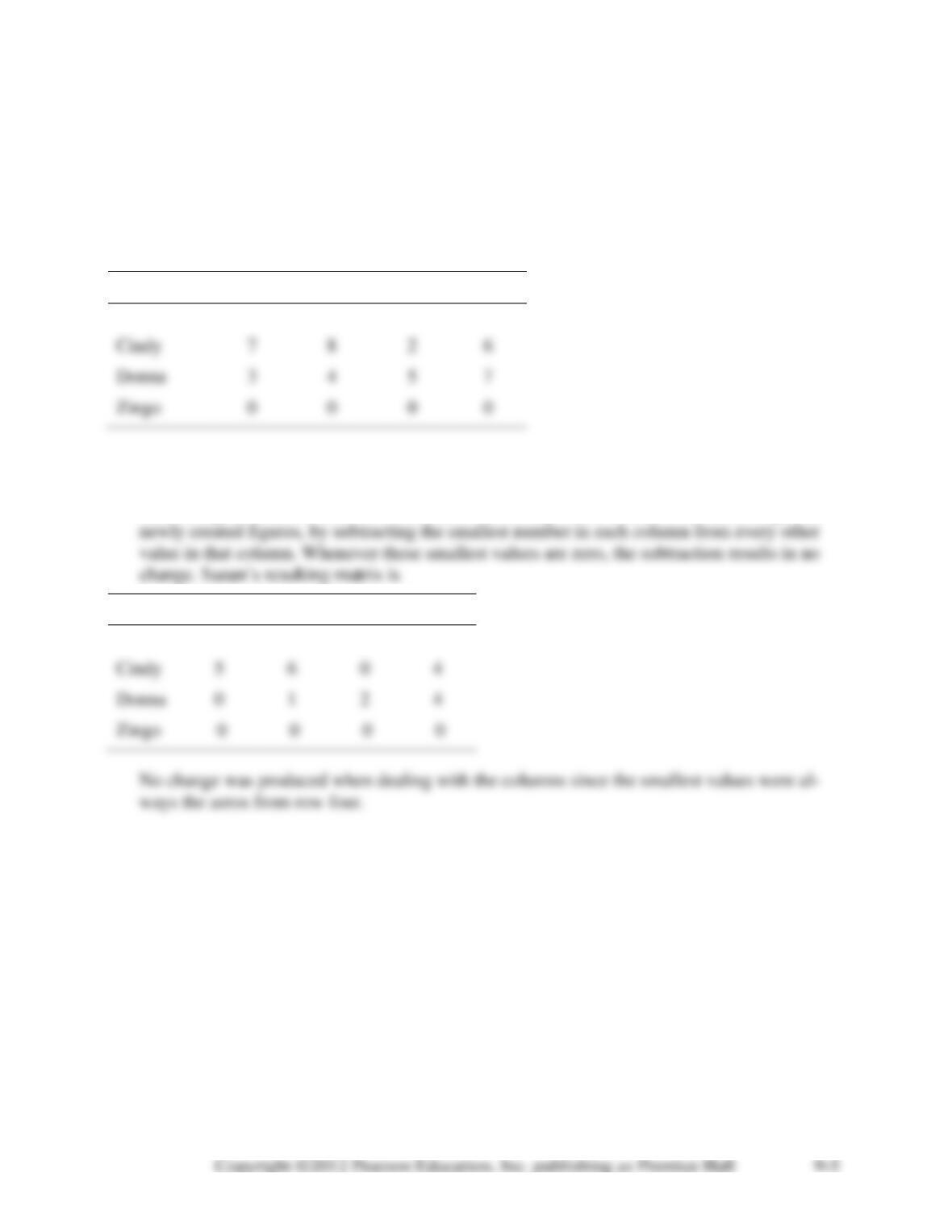
Alternative Example 9.4: As an example of an assignment problem, let us assume that Susan is
a sorority pledge coordinator with four jobs and only three pledges. Susan decides that the as-
signment problem is appropriate except that she will attempt to minimize total time instead of
money (since the pledges aren’t paid). Susan also realizes that she will have to create a fictitious
fourth pledge and she knows that whatever job gets assigned to that pledge will not be done (this
semester, anyhow). She creates estimates for the respective times and places them in the follow-
ing table:
Job 1
Job 2
Job 3
Job 4
Barb
4
9
3
8
Cindy
7
8
2
6
Zingo
0
0
0
0
Zingo is, of course, a fictitious pledge, so her times are all zero.
(a) The first step in this algorithm is to develop the opportunity cost table. This is done by
subtracting the smallest number in each row from every value in that row, then, using these
Job 1
Job 2
Job 3
Job 4
Barb
1
6
0
5
Cindy
5
6
0
4
Donna
0
1
2
4
Zingo
0
0
0
0
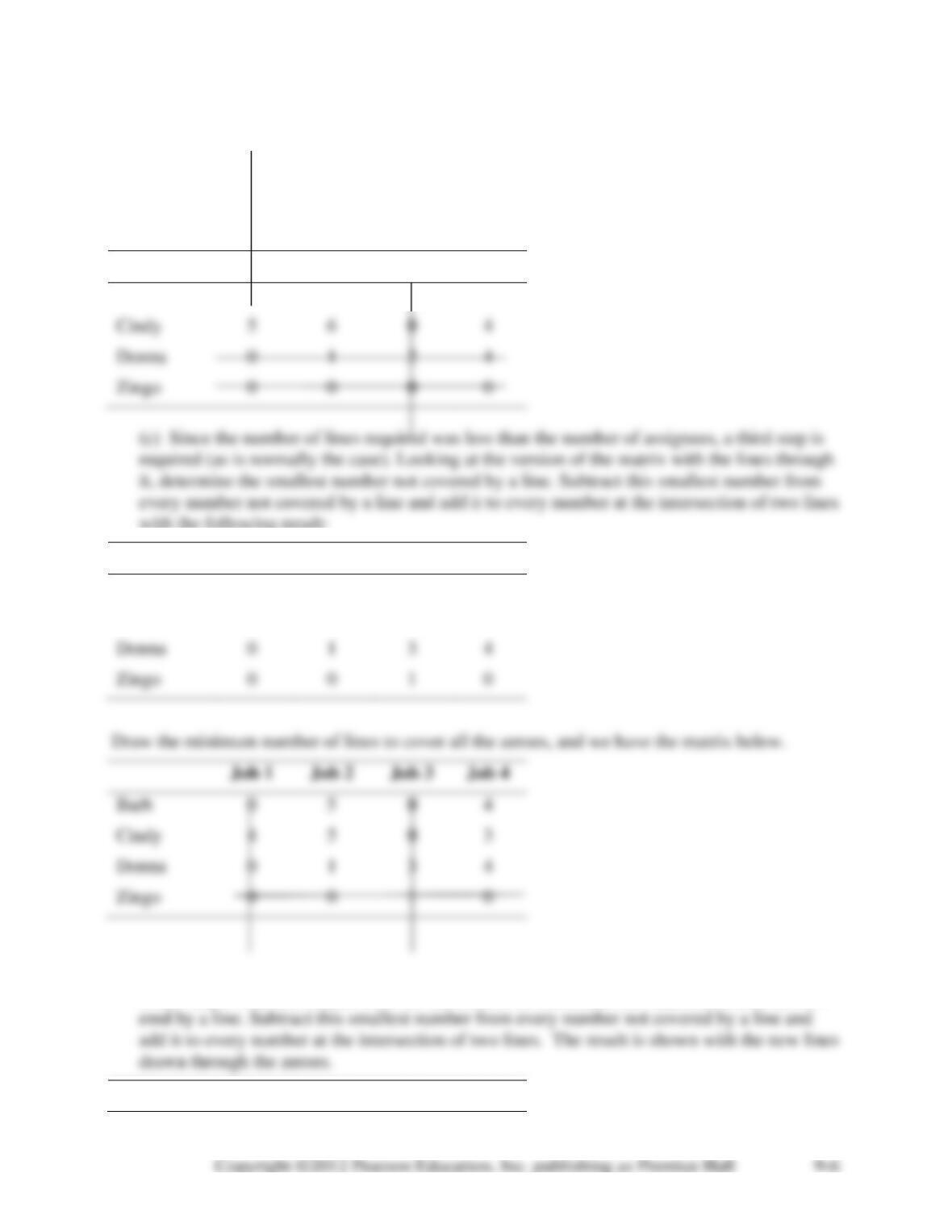
(b) The next step is to draw lines through all of the zeros. The lines are to be straight and ei-
ther horizontal or vertical. Furthermore, you are to use as few lines as possible. If it requires
four of these lines (four because it is a 4 4 matrix), an optimal assignment is already possi-
ble. If it requires fewer than four lines, another step is required before optimal assignments
may be made. In our example, draw a line through: row four, column three, and either col-
umn one or row three. One version of the matrix is
Job 1
Job 2
Job 3
Job 4
Barb
1
6
0
5
Cindy
5
6
0
4
Donna
0
1
2
4
Zingo
0
0
0
0
with the following result:
Job 1
Job 2
Job 3
Job 4
Barb
0
5
0
4
Cindy
4
5
0
3
Donna
0
1
3
4
Zingo
0
0
1
0
Job 1
Job 2
Job 3
Job 4
Barb
0
5
0
4
Cindy
4
5
0
3
Donna
0
1
3
4
Since only 3 lines are needed to cover the zeroes, we determine the smallest number not cov-
Job 1
Job 2
Job 3
Job 4
Barb
0
4
0
3
Cindy
4
4
0
2
Donna
0
0
3
3
Zingo
1
0
2
0
(d) Since this matrix requires four lines to cover all zeros, we have now reached an optimal
solution stage.
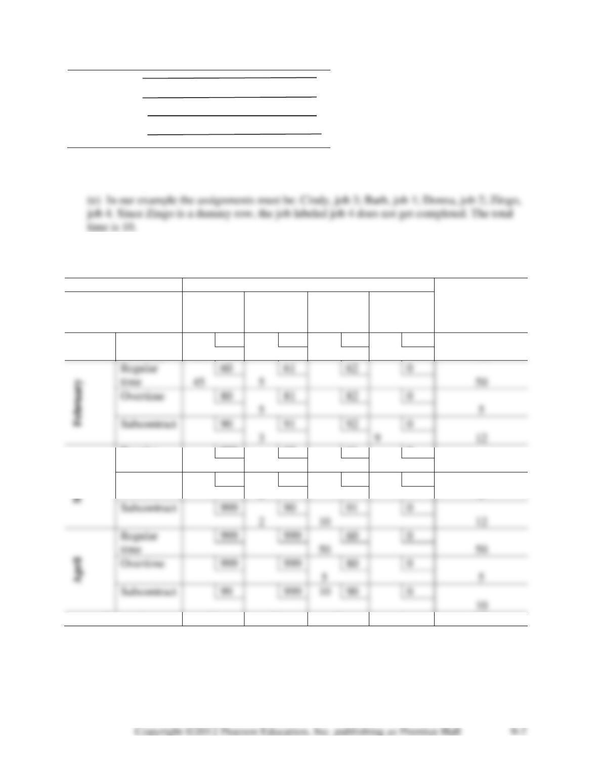
Table for Alternative Example 9.3:
Transportation Solution
Demand for:
Total Capacity
Available (Sup-
ply)
Supply from:
Feb.
Mar.
Apr.
Unused
Capacity
(Dummy)
Pe-
ri-
od
Beginning
inventory
0
3
2
0
10
10
Regular
time
60
61
62
0
50
45
5
80
81
82
0
5
5
Subcontract
90
91
92
0
12
3
9
Subcontract
999
90
91
0
12
2
10
Regular
time
999
999
60
0
50
50
999
999
80
0
5
5
Subcontract
99
999
10
90
0
10
Regular
time
999
60
61
0
50
50
Overtime
999
80
81
0
5
5
Demand
55
70
75
9
209
SOLUTIONS TO DISCUSSION QUESTIONS AND PROBLEMS
9-1. The transportation model is an example of decision making under certainty where a deci-
9-2. In a transportation problem, each source-destination pair represents a decision variable.
Hence, to determine the total number of decision variables one would need only multiply the
9-3. A balanced transportation problem is one in which total demand (from all destinations) is
9-4. This would cause two filled cells to become empty simultaneously. This means that the so-
lution in the next table will be degenerate. Placing a 0 in one of these two cells and treating this
as a filled cell can resolve this difficulty.
9-5. The total cost will decrease $2 for each unit that is placed in this empty cell. Since the max-
9-6. When m + n − 1 squares (where m = number of rows and n = number of columns) are not
9-7. The enumeration method (determining all possible combinations) is not a practical means
9-8. The assignment problem is a special case of the transportation problem and hence can be
solved with the approach shown earlier in this chapter. This is illustrated for the Fix-It Shop
problem. Notice that the column and row requirements will always be equal to 1.
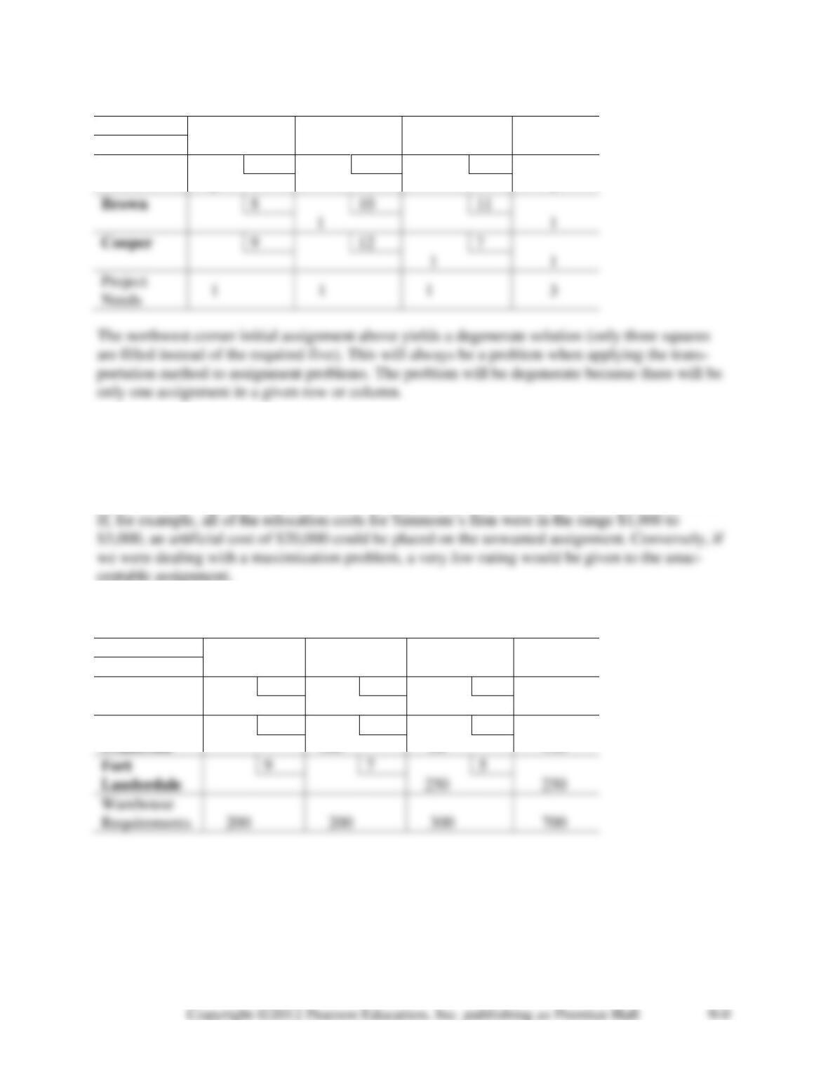
To
Project
1
Project
2
Project
3
Personnel
Available
FROM
Adams
$11
$14
$6
1
1
Brown
8
10
11
1
1
Cooper
9
12
7
1
Needs
9-9. It is not necessary to rework the assignment solution. Changing each entry in the cost table
will not result in different total opportunity cost tables. The optimal cost will, however, be in-
creased by $25 from $492 to $517 because of the extra $5 charge for each of the five workers.
9-10. To exclude any unwanted or unacceptable assignment from occurring, it is necessary only
to place a very high artificial cost in the row and column representing that particular assignment.
9-11. a. Initial solution to modify Executive Furniture Corporation problem using the northwest
corner rule:
To
Albu-
querque
Boston
Cleveland
Factory
Capacity
FROM
Des Moines
5
4
3
300
200
100
Evansville
8
4
3
150
100
50
9
7
5
Requirements
700
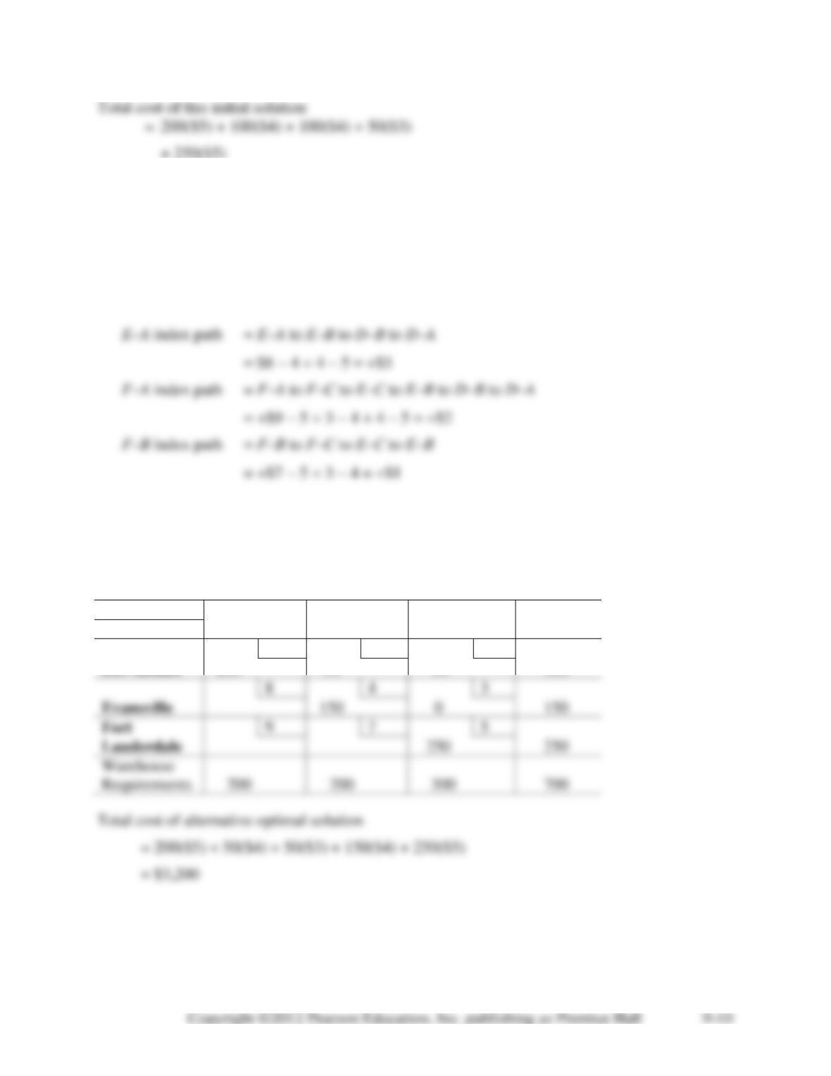
= 1,000 + 400 + 400 + 150 + 1,250
= $3,200
b. To see if this initial solution is optimal, we compute improvement indices for each unused
square, namely, D–C, E–A, F–A, and F–B:
D–C index path = D–C to E–C to E–B to D–B
= $3 − 3 + 4 − 4 = $0
This solution is optimal, so further stepping–stone computations are not necessary.
c. The improvement index for square D–C is zero. This implies the presence of multiple op-
timal solutions. Practically speaking, management could close the E–C shipping route and
send 50 units on the D–C route instead. The table below illustrates the overall changes in this
alternative optimal solution.
To
Albu-
querque
Boston
Cleveland
Factory
Capacity
FROM
Des Moines
5
4
3
300
200
50
50
Evansville
8
4
3
150
150
9
7
5
250
Requirements
700
9-12. Let AD, AE, AF, BD, BE, BF, CD, CE, and CF represent the amounts shipped from Albu-
querque, Boston, and Cleveland to Des Moines, Evansville, and Fort Lauderdale respectively.
The associated linear program can be formulated as follows:
Minimize costs: 5AD + 8AE + 9AF + 4BD + 4BE + 7BF + 3CD + 3CE + 5CF
subject to:
AD + AE + AF = 200
BD + BE + BF = 200
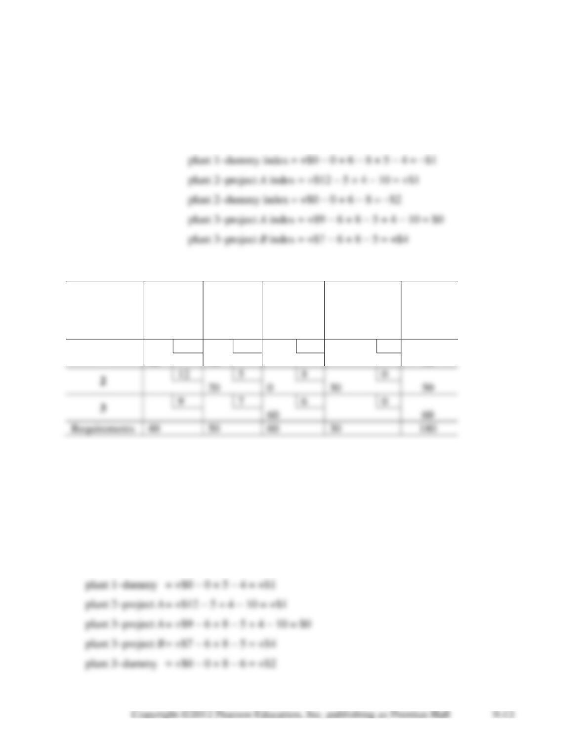
9-13. a. Hardrock’s initial solution using the northwest corner rule is shown below.
To
A
B
C
Plant
Capacity
FROM
1
10
4
11
70
40
30
12
5
8
50
20
3
9
7
6
30
quirements
Using the stepping-stone method, the following improvement indices are computed:
plant 1–project C = $11 − $4 + $5 − $8 = +$4
(closed path: 1-C to 1-B to 2-B to 2-C)
plant 2–project A = +$12 − $5 + $4 − $10 = $1
(closed path: 2-A to 2-B to 1-B to 1-A)
b. There is an alternative optimal solution to this problem. This fact is seen by the index for
plant 3–project A being equal to zero. The other optimal solution, should you wish for students to
pursue it, is as follows:
plant 1–project A = 20 units
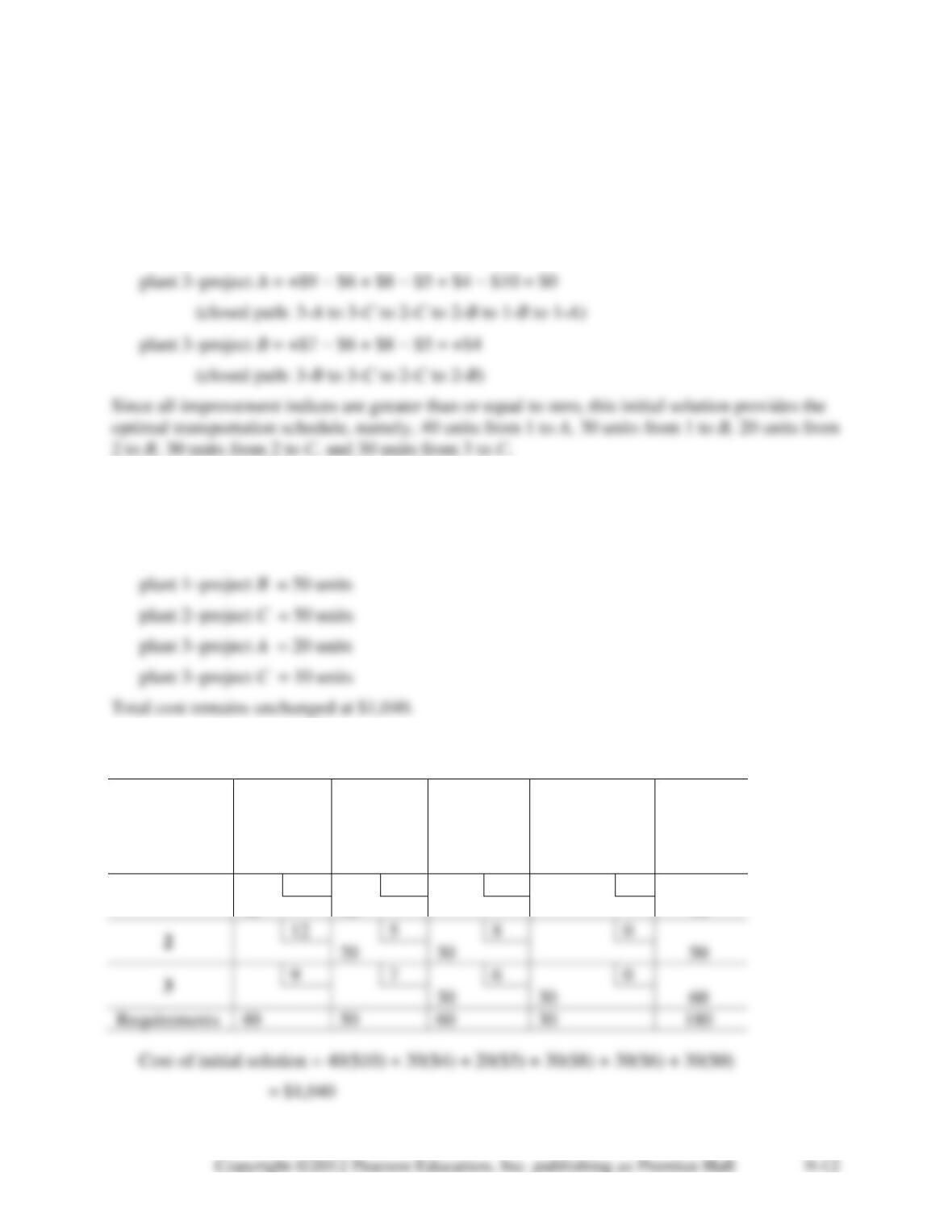
9-14. Hardrock’s problem now requires the addition of a dummy project (destination) because
supply exceeds demand. The northwest corner initial solution is as follows:
TO
FROM
A
B
C
Dummy
Capacity
1
10
4
11
0
70
40
30
12
5
8
0
50
20
30
9
7
6
0
60
30
30
40
50
60
30
This is the same initial assignment and cost as that found in Problem 9-13. This coincidence oc-
curs because the change in plant capacity is at the lower right-hand corner of the table and is un-
affected by the northwest corner rule.
plant 2–project A index = +$12 − 5 + 4 − 10 = +$1
plant 3–project A index = +$9 − 6 + 8 − 5 + 4 − 10 = $0
Testing the unused routes:
plant 1–project C index = $11 − 8 + 5 − 4 = +$4
The second table involves bringing the plant 2–dummy route into the solution as follows:
TO
FROM
A
B
C
Dummy
Capacity
1
10
4
11
0
70
40
30
2
12
5
8
0
50
20
0
30
9
7
6
0
60
60
40
50
60
30
Cost of this iteration = $980.
Because two squares became zero by opening the plant 2–dummy route, the current solution is
degenerate (fewer than 3 rows + 4 columns − 1 square are occupied). We will need to place an
artificial zero in an unused square (such as plant 2–project C) to be able to trace all of the closed
paths and evaluate whether this solution is optimal.
We now trace the closed paths for the six unused squares (we assume that the plant 2–project
C square has a zero in it). The indices are:
plant 1–project C = +$11 − 8 + 5 − 4 = +$4
Since all indices are zero or positive, an optimal solution has been reached. Again, note that the
plant 3–project A route has an improvement index of $0, implying that an alternative optimal so-
lution exists. The alternative optimal solution, whose total cost is also $980, is shown in the fol-
lowing table.
TO
FROM
A
B
C
Dummy
Capacity
1
10
4
11
0
70
20
50
12
5
8
0
9
7
6
0
60
20
40
40
50
60
30
9-15. Let A1, A2, A3, B1, B2, B3, C1,C2, and C3 represent the amounts delivered to projects A, B,
and C from plants 1, 2, and 3 respectively. The associated linear program is formulated as follows:
Minimize costs: 10A1 + 12A2 + 9A3 + 4B1 + 5B2 + 7B3 + 11C1 + 8C2 + 6C3
subject to:
A1 + A2 + A3 = 40
{All variables} ≥ 0
The solution is: total cost = 1040; A1= 20; A2= 0; A3= 20; B1= 50; B2= 0; B3= 0; C1= 0;C2=
50; and C3= 10. Multiple optimal solutions exist.
9-16. a. Using the northwest corner rule for the Saussy Lumber Company data, the following
initial solution is reached:
To
Customer
1
Customer
2
Customer
3
Capacity
FROM
Pineville
3
3
2
25
25
Oak Ridge
4
2
3
40
30
Mapletown
3
2
3
30
Demand
95
= $260
b. Applying the stepping-stone method, the improvement indices are computed:
Mapletown–customer 1 = +$3 − 3 + 3 − 4 = −$1
best
Pineville–customer 2 = +$3 − 2 + 4 − 3 = +$2
Pineville–customer 3 = +$2 − 3 + 4 − 3 = $0
The improved solution is shown in the following table. Its cost is $255.
To
Customer
1
Customer
2
Customer
3
Capacity
FROM
Pineville
3
3
2
25
25
Oak Ridge
4
2
3
40
30
Mapletown
3
2
3
30
Checking improvement indices again, we find that this improved solution is still not optimal. The
improvement index for the Pineville–customer 3 route = +$2 − 3 + 3 − 3 = −$1. Hence another
shift is necessary. The third iteration is shown in the following table:
To
Customer
1
Customer
2
Customer
3
Capacity
FROM
Pineville
4
2
3
Mapletown
3
2
3
Demand
3
3
2
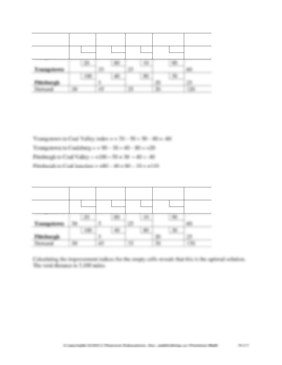
9-17. Krampf Lines Railway Company’s initial northwest corner solution is shown below.
TO
FROM
Coal
Valley
Coaltown
Coal
Junction
Coalsburg
Supply
Morgantown
50
30
60
70
35
30
5
Youngstown
60
40
20
Pittsburgh
100
40
80
30
25
5
20
Demand
30
45
25
20
120
20
80
10
90
To test for improvement with the stepping stone method, we determine the improvement index
for each unoccupied square. These are:
Morgantown to Coal Junction = +60 – 10 + 80 – 30 = +100
Morgantown to Coalsburg index = +70 – 30 + 80 – 10 + 80 – 30 = +160
Youngstown to Coal Valley index = + 20 – 50 + 30 – 80 = -80
TO
FROM
Coal
Valley
Coaltown
Coal
Junction
Coalsburg
Supply
Morgantown
50
30
60
70
35
30
5
Youngstown
20
80
10
90
60
35
25
Pittsburgh
100
40
80
30
25
5
20
Demand
30
45
25
20
120
Evaluating the empty cells with the steppingstone method, we get the following improvement
indices:
Morgantown to Coal Junction = +60 – 10 + 80 – 30 = +100
Morgantown to Coalsburg index = +70 – 30 + 40 – 30 = +50
The best improvement index is -80 from Youngstown to Coal Valley. Filling this cell and modi-
fying those cells on the steppingstone path we get:
TO
FROM
Coal
Valley
Coaltown
Coal
Junction
Coalsburg
Supply
Morgantown
50
30
60
70
35
35
Youngstown
20
80
10
90
60
30
5
25
Pittsburgh
100
40
80
30
25
5
20
Demand
30
45
25
20
120
9-18. Let MCV, MCT, MCJ, MCB, YCV, YCT, YCJ, YCB, PCV, PCT, PCJ, and PCB represent
the amounts shipped from Morgantown, Youngstown, and Pittsburgh to Coal Valley, Coaltown,
Coal Junction, and Coalsburg respectively. The associated linear program is formulated as fol-
lows:
Minimize costs: 50MCV + 30MCT + 60MCJ + 70MCB + 20YCV + 80YCT + 10YCJ +
90YCB + 100PCV + 40PCT + 80PCJ + 30PCB
subject to:
The optimal solution found using the computer is:
total cost = 3100; MCV = 0; MCT = 35; MCJ = 0; MCB = 0; YCV = 30; YCT = 5; YCJ = 25;
YCB = 0; PCV = ;0 PCT = 5; PCJ = 0; and PCB = 20.
9-19. Because of the excess factory capacity, a dummy destination (column) is added to the
problem before starting. The solution shown below is one optimal solution.
To
Dallas
Atlanta
Denver
Dummy
Factory
Capacity
FROM
Houston
8
12
10
800
10
14
9
250
11
8
12
300
9-20. Let HDA, HAT, HDE, PDA, PAT, PDE, MDA, MAT, AND MDE represent the amounts
shipped from Houston, Phoenix, and Memphis to Dallas, Atlanta, and Denver. Notice that the
dummy destination can be ignored. The associated linear program can be formulated as follows:
Minimize costs: 8HDA + 12HAT + 10HDE + 10PDA + 14PAT + 9PDE + 11MDA +
8MAT + 12MDE
subject to:
The optimal solution found using the computer is: total cost = 14,700; HDA = 800; HAT = 50;
HDE = 0; PDA = 0; PAT = 250; PDE = 200; MDA = 0; MAT = 300; and MDE = 0.
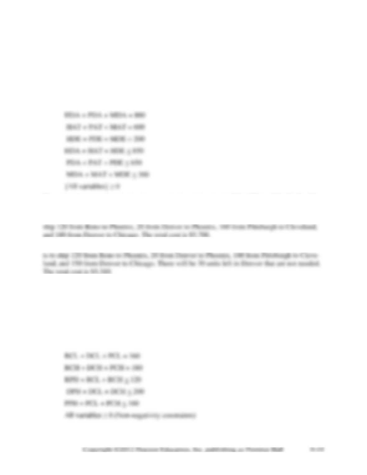
9-21. The optimal solution found using computer software for the transportation algorithm is to
9-22. The problem is unbalanced and a dummy destination must be added. The optimal solution
9-23. Let RPH, RCL, RCO, DPH, DCL, DCH, PPH, PCL, and PCH represent the tables deliv-
ered from Reno, Denver, and Pittsburgh to Phoenix, Cleveland, and Chicago respectively. The
associated linear program can then be formulated as follows:
Minimize costs: 10RPH + 16RCL + 19RCH +12DPO + 14DCL + 13DCH + 18PPH +
12PCL + 12PCH
subject to:
RPH + DPH + PPH = 140
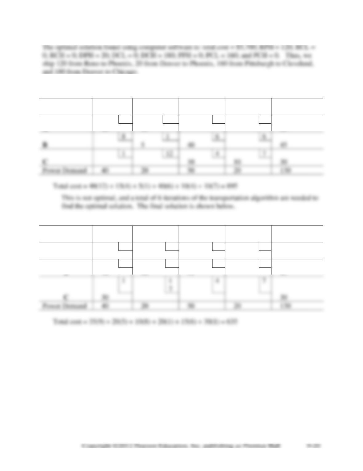
9-24. a. An initial solution using the northwest corner method is as follows:
TO
Excess
FROM
W
X
Y
Z
Supply
12
4
9
5
A
40
15
55
8
1
6
6
B
5
40
45
1
12
4
7
C
10
10
30
Power Demand
40
20
50
20
130
TO
Excess
FROM
W
X
Y
Z
Supply
12
4
9
5
A
35
20
55
8
1
6
6
B
10
20
15
45
2
C
30
30
Power Demand
40
20
50
20
130